3. Selected Nordic cities and model grids

This chapter includes a description of the selected Nordic cities, their city boundaries and related model grids.

Based on the number of inhabitants in the largest cities in the Nordic countries, three cities were selected in each country except for Iceland as shown in Table 3.1. The number of inhabitants is from Eurostat data based on a 1 km x 1 km grid and selected within the city boundaries. As a starting point the three largest cities were selected. However, it has also been an objective to ensure larger cities in different parts of the countries.

For Finland the second (Espoo) and fourth (Vanta) largest cities are part of the Helsinki urban region and hence Tampere (3^rd) and Oulu (5^th) were chosen.

Reykjavík urban region is considered one urban area consisting of six contiguous municipalities, Reykjavík, Kópavogur, Garðabær, Hafnarfjörður, Seltjarnarnes and Mosfellsbær. It could be considered as Greater Reykjavík. Other cities on Iceland are small, and for small cities, the urban background concentration over the city will be almost entirely dominated by the regional background concentrations and sources in the city will have very limited influence on urban background concentrations. Therefore, only Greater Reykjavík has been chosen for Iceland.

Table 3.1. Selection of largest cities in each of the Nordic countries. Inhabitants based on Eurostat within city boundaries.

For the Danish cities the population by Eurostat was compared with population data from Statistics Denmark. Eurostat estimates 548,000 inhabitants in 2018 based on the gridded data for København following the administrative boundaries. Statistics Denmark indicates 718,000 inhabitants for the municipalities of København and Frederiksberg or a difference of 24%. It was unexpected to find such large difference adding to the uncertainty on estimation of health effects and related external costs. For Aarhus and Odense the differences were within 2%. The data from Eurostat was chosen for all Nordic cities for consistency throughout the project.

The location of the selected cities is seen in Figure 3.1.

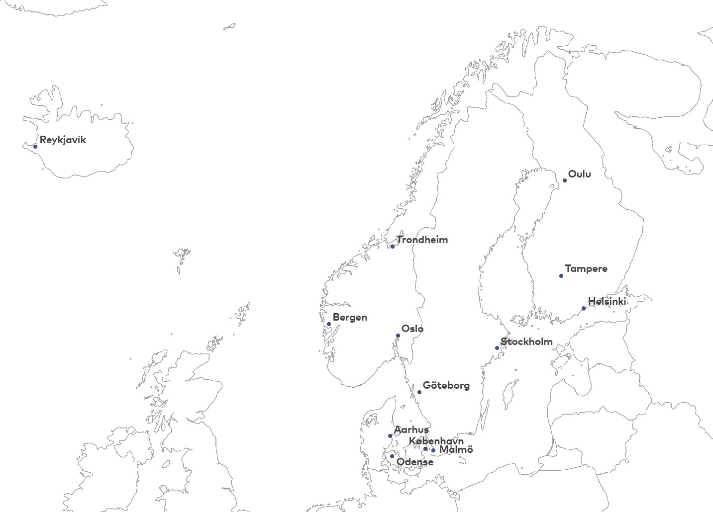
Figure 3.1.  The location of the selected Nordic cities.

The definition of city boundaries is not well-defined as it depends on what is considered to belong to the city.

A standardized approach was used across the Nordic countries to define the boundaries of cities based on the EC-OECD city definition used for the Eurostat Urban Audit data collection. These datasets include boundaries for cities, greater cities and functional urban areas defined in the following way. A City is a local administrative unit (LAU) where the majority of the population lives in an urban centre of at least 50,000 inhabitants. The Functional Urban Area consists of a city and its commuting zone, formally known as larger urban zone (LUZ). The Greater City is an approximation of the urban centre when this stretches far beyond the administrative city boundaries.

The different city boundaries are illustrated in Figure 3.2.

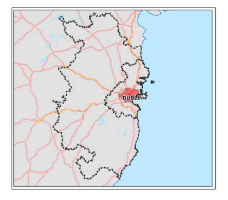
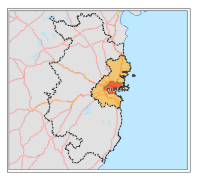
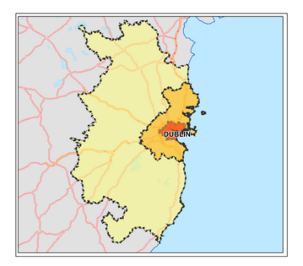
Figure 3.2. Illustration of different city boundaries with the case of Dublin (Source: Eurostat).

Based on an analysis of the three different types of city boundaries, the most suitable type of boundary is the city boundary for the selected cities. The city boundaries are based on administrative boundaries of the city.

Although the same city boundary type was chosen for all cities, they are still quite different with respect to geographical extend and how much is built-up urban area and how much is rural/natural area. In Appendix 1 the city boundaries are shown on aerial photos. Examples of cities that are almost entirely composed of built-up urban areas are København, Stockholm, Helsinki and Malmö where the rest of the cities have larger rural/natural areas outside the urban built-up area within the administrative city boundary.

One of the outcomes of the modelling is an average concentration in 2030 over the area defined by the city boundaries. It is obvious that an area with a city boundary which almost entirely includes built-up area will have higher concentrations than an area with a city boundary that includes large rural/natural areas, due to the differences in emission density. This should be kept in mind when comparing results from different cities.

It is also evident that Eurostat doesn’t characterize suburban areas as a specific part of cities. Therefore, it has not been possible to e.g. analyse the average concentration over suburban areas or their contribution to city concentrations.

It is necessary to define receptors for the UBM model over the selected cities to be able to calculate the average concentration over the areas defined by the city boundaries, and to be able to calculate the contribution to the average concentration of the emissions within the city boundaries.

The regional model (DEHM) provides the background concentrations to the cities and the urban background model (UBM) calculates the local contribution taking into account the upstream background concentration from 25 km upstream and the emissions 25 km upstream and to the receptor point in question. The upstream area is illustrated in Figure 3.3 for København.

The EEA reference grid on a 1 km x 1 km resolution is used for the Nordic countries. The coordinate reference system (CRS) for the EEA reference grid is ETRS89/LAEA Europe. The Geodetic Datum is the European Terrestrial Reference System 1989. The Lambert Azimuthal Equal Area (LAEA) projection is centred at 10E, 52N. Being based on an equal area projection, the EEA reference grid is suitable for generalising data, statistical mapping and analytical work whenever a true area representation is required (EEA, 2011).

The upstream area for København is illustrated in Figure 3.3.

Figure 3.3. Upstream area for København shown as a schematic 25 km circle around København. Municipal boundaries are shown for part of Zealand in Denmark. Schematic country boundaries are also shown. The city grid for København is also shown (beige area).

The city grid for København is illustrated in Figure 3.4.

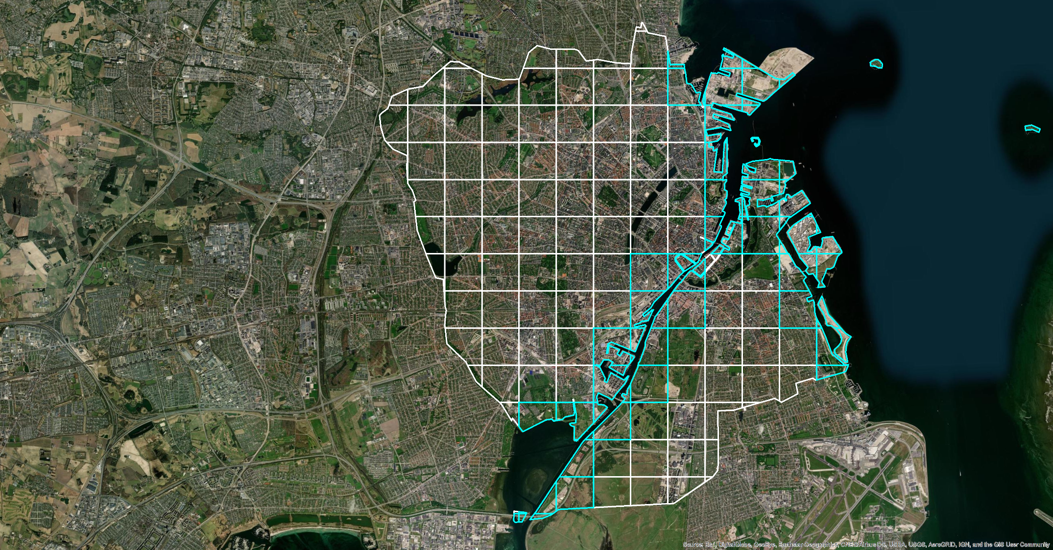
Figure 3.4. City grid for København. Grid size as rectangle 13 km x 15 km. Grid cells are visualized and those bordering water are highlighted.

The city grid serves both as receptor grid, emission grid and population grid. The receptor grid includes the receptor points for the UBM calculations as the centre point of each grid cell (centre in 1 km x 1 km cell). The grid cell is also used to calculate the number of inhabitants for health impact calculations based on the share of the area of the cell that is within the city boundaries as information of inhabitants are based on the 1 km x 1 km grid cells. Similar for emissions where the share of the area of the cell that is within the city boundaries is used to assign emissions to the cell. In the case that a grid cell is bordering water, then the entire emission and inhabitants of the grid cell are used.

For each of the selected cities the receptor grid and emission grid has been prepared and the shares of areas of the cells within the city boundaries as well as cells bordering water have been identified using GIS techniques.

In Table 3.2, a description of the extend of city grid size and upstream grid as rectangles is shown.         

Table 3.2. Description of the extend of each city, the grid size and the upstream grid as rectangles.