4. Modelling historical and future conditions in Limfjorden

Limfjorden is a shallow fjord with an average depth of 4.8 meters, consisting of several smaller basins connected by narrow straits (Fig. 14). It is located in the northern part of Denmark, with connections to the North Sea to the west and the fresher Kattegat to the east. Therefore, the salinity in the fjord varies from 32–34 psu in the west to 19–24 psu in the east (Fig. 14). Additionally, there is low salinity in basins with high freshwater inflow. The main current flows from west to east, modified by wind direction and a weak tidal signal (Schourup-Kristensen et al. 2021). Limfjorden has high concentrations of nutrients with seasonal oxygen depletion (hypoxia) in the inner basins and a high population of blue mussels (Maar et al. 2023a, Schourup-Kristensen et al. 2023). The system receives nutrients from freshwater sources, as the catchment area is dominated by agriculture, and the fjord is therefore in poor ecological condition according to the EU Water Framework Directive. Limfjorden is the most important area for mussel fishing and -farming in Denmark. Mussel dredging is currently the most important type of fishing, as the fish stocks in the fjord collapsed in the 1990s. Since then, mussel catches have fallen from about 122 Kt wet weight in 2001 to 20 Kt wet weight in 2022 (data from the Danish Fisheries Agency). However, mussel harvests from commercial farms have increased from very low numbers in 2009–2017 to 8.4 Kt wet weight in 2022 due to higher technological expertise and good profitability. The number has not increased in very recent years though, due to a temporary ban on new permits. Still, the number of applications is about the same as the number of current farms, so when the government approves new permits, growth is expected. Additionally, Limfjorden is an important area for tourism and recreational activities.

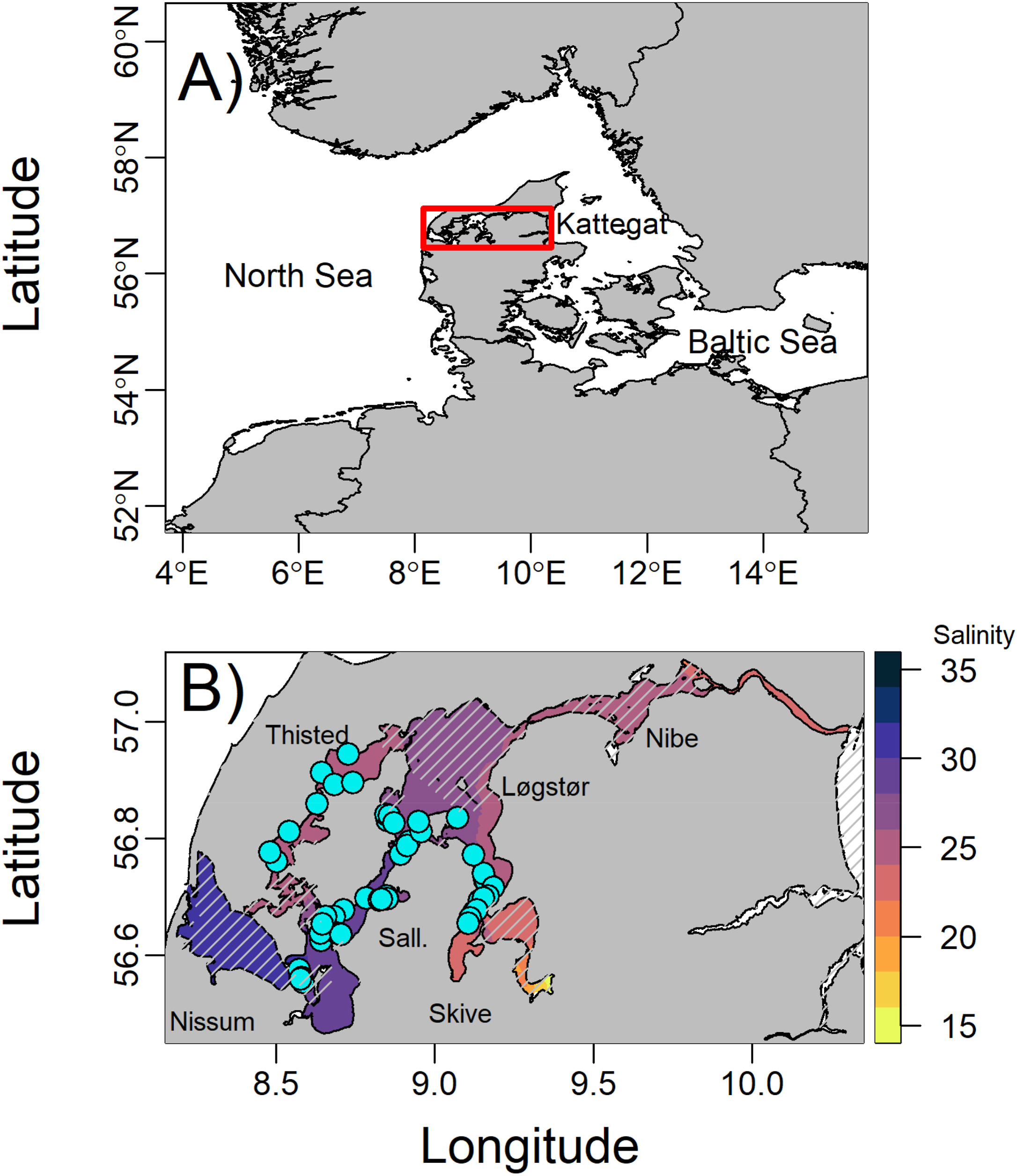
Figure 14. A) Limfjorden (red box) is located in the northern part of Denmark between the North Sea and Kattegat and B) modelled surface salinity (color bar), mussel farms (cyan points), and names of the main basins; Nissum Broad (Nissum), Sallingsund (Sall.), Thisted Broad (Thisted), Løgstør Broad (Løgstør), Skive Fjord (Skive), and Nibe Broad (Nibe). Grey hatched lines are the Natura 2000 areas where mussel farming is not allowed. From Maar et al. (2024).

The FlexSem model has been set up in a 3D coupled hydrodynamic-biogeochemical model for Limfjorden (Larsen et al. 2020, Maar et al. 2024). The model used an unstructured grid with 6, 686 elements covering a total area of 1,502 km² (Fig. 15). The size of the elements varied from 143 m to 1,773 m with an average of 474 m. The vertical resolution was 1.5 m in the flexible surface layer, followed by nine 1 m depth layers and three 5 m layers, with a maximum water depth of 30 m. The hydrodynamic model solved the Navier-Stokes equations for velocities and the advection-diffusion equations for the transport of tracers (e.g., heat, salinity, nutrients). The turbulent part of the hydrodynamic solution was modelled using a k-epsilon model in the vertical and a Smagorinsky model in the horizontal. A surface radiation model calculated heat transfer through the sea surface and changed the water temperature.

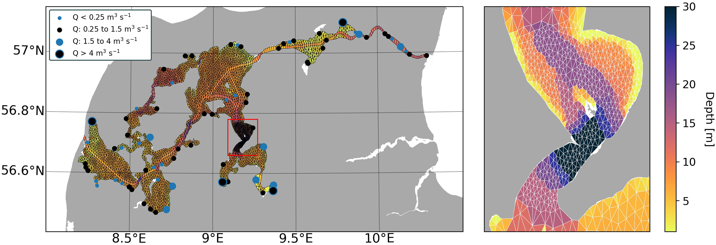
Figure 15. The FlexSem model setup for Limfjorden shows water depth (colour scale), elements (grey polygons), and freshwater sources categorized by size (blue/black circles). The panel on the right is a close-up of the area within the red square on the left. From Schourup-Kristensen et al. (2021).

The hydrodynamic model was fully coupled to a biogeochemical model, which includes a water phase model, coupled to a sediment model and a mussel model (Maar et al. 2023a, 2024). The model describes the state and changes in nutrients (nitrate, ammonium, phosphate), phytoplankton (picoplankton, flagellates, diatoms), micro- and mesozooplankton, detritus, oxygen, bottom-dwelling mussels, small animals in the sediment, and sediment pools of nutrients over time and space (Fig. 16). The described processes include nutrient uptake, growth, grazing, mortality, respiration, nutrient excretion, sedimentation, resuspension, detritus decomposition, nitrification, denitrification, diffusion between the water column and sediment, and nutrient regeneration. The mussel model is a dynamic energy budget model that describes the ecophysiological growth of mussels in a mussel farm and feedback mechanisms to the ecosystem (Fig. 16).

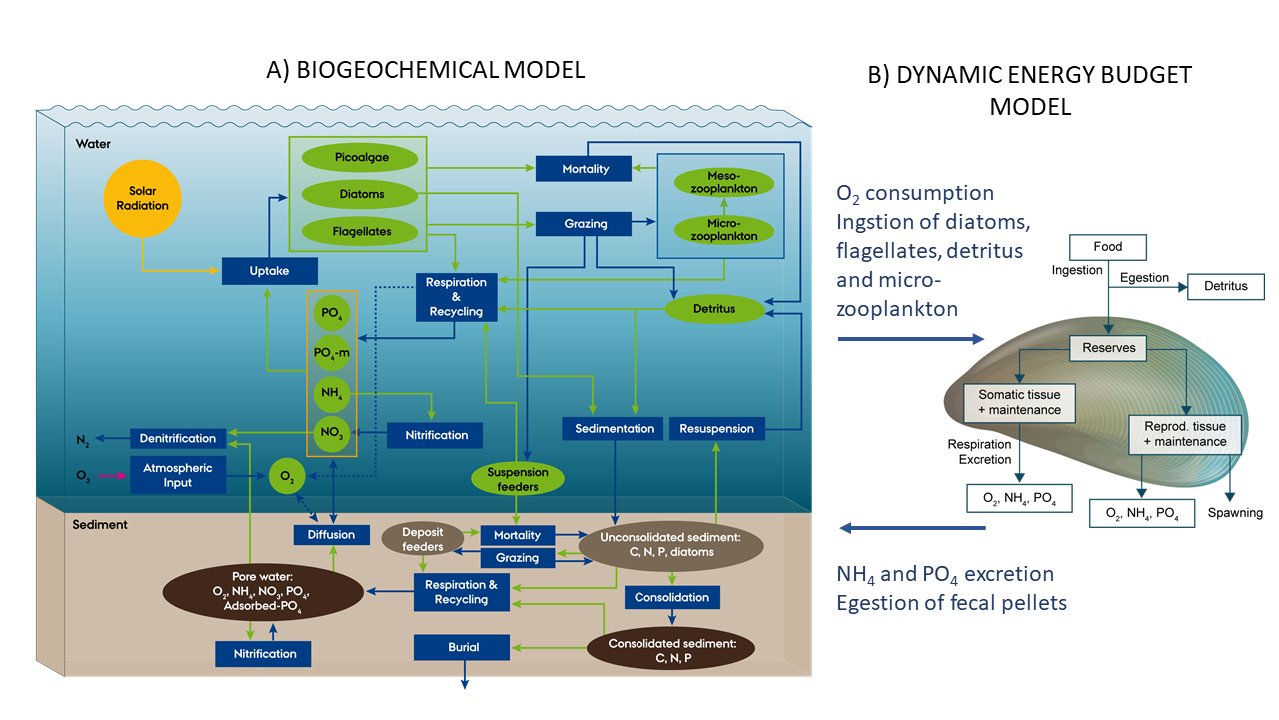
Figure 16. Conceptual model diagram of the biogeochemical model applied in FlexSem for Limfjorden. The blue background represents the water column and the brown background the sediment. The green and brown ovals show the state variables in the water column and sediment, respectively, and the blue boxes represent ecosystem processes. The biogeochemical model is two-way coupled to a dynamic energy budget mussel model. Extended from Schourup-Kristensen et al. (2023).

The reference scenario in Limfjorden used historical data (2009 to 2018) for atmospheric pressures, open boundary conditions, and freshwater runoff. Atmospheric data were taken from the EC-Earth CMIP6 simulations, as they showed the best quality in the study area (Kristiansen & Butenschön 2023). Limfjorden has two open boundaries, one towards the North Sea and one towards Kattegat. Values for salinity, temperature, water level, and current speeds at the two open boundaries were provided by the HIROMB-BOOS-HIRLAM model (Murawski et al. 2021). Boundary values for nutrients, Chl a (distributed in the three phytoplankton groups), and oxygen were obtained from monitoring data (https://odaforalle.au.dk/). Runoff (diffuse and point sources) and nutrient input (TN=total nitrogen and TP=total phosphorous) were obtained from the SWAT catchment model with 79 sources with daily resolution (Molina-Navarro et al. 2017). There were 14 active commercial mussel farms, which represents the average mussel production in the reference period.

IPCC works with a set of different scenarios for future greenhouse gas emissions and thus the future climate of the planet. In this study, EC-Earth CMIP6 simulations were used, as the downscaled CMIP7 products were not yet available when the study was conducted. The three climate scenarios used (SSP1-2.6, SSP2-4.5, and SSP5-8.5) are named after different socio-economic developments (SSP) and the level of radiative forcing in the year 2100 of 2.6, 4.5, and 8.5 W/m², respectively (Table 3). SSP1-2.6 is largely consistent with the maximum atmospheric CO₂ concentration required under the Paris Agreement, which aims to “significantly reduce global greenhouse gas emissions to limit the global temperature increase this century to 2 °C while pursuing efforts to limit the increase even further to 1.5 °C.”

Greenhouse gas emissions are partially higher in SSP2-4.5, while they continue to rise throughout the whole 21^st century in SSP5-8.5. The scenarios were conducted for the periods 2051–2060 and 2090–2099. There was a spin-up period of 10 years to achieve semi-stable conditions for the water column and sediment. A statistical downscaling of several sea models for the North Sea was used to create monthly average values for temperature, salinity, Chl a, and oxygen for boundary data in the scenarios (Kristiansen & Butenschön 2023), while all other variables remained unchanged from the reference period. The SWAT catchment model made future runs under the three scenarios to calculate future runoff and nutrient load.

In the SSP1-2.6 and SSP2-4.5 scenarios, it was also assumed that reductions in land-based nutrient loads were implemented according to the Danish water plans (36% reduction of the current N load, no P reduction required) (Danish Ministry of Environment and Food 2016). In the SSP5-8.5 scenario, it was assumed that the national water plans were not implemented due to the growth of the agricultural sector with little regard for environmental impacts (Table 3). We assumed that mussel production would be intensified (52 commercial mussel farms) to meet the global market demand for protein foods with a low CO₂ footprint in all scenarios after consultation with stakeholders in the EU FutureMARES project.

Table 3. Overview of model reference period and future scenarios with time periods, number of mussel farms, degree of reduction of nitrogen supply, implementation of water plans, and emission level.

The shallow Limfjord is characterized by a salinity of approximately 32–34 psu in the western part, connected to the North Sea, and lowest in the innermost part of the fjord where there is high runoff (20 psu, Fig. 17). Surface temperatures also show a gradient with slightly warmer water towards the west and cooler water towards the east and in the innermost part (Fig. 18).

Before the model is applied for the future, it is important to verify that it works well for present and historical times. For model verification we apply so-called Taylor diagrams, which indicate correlation coefficient, bias, and the normalized standard deviation, nSD, between the model and observation-based data. Results with a high correlation, low bias, and an nSD within 1±25% show the best representation of the measurement data. Comparison with measurements in the reference period shows good agreement both seasonally, between years, and spatially between stations for both salinity and temperature (Figs. 17 and 18).

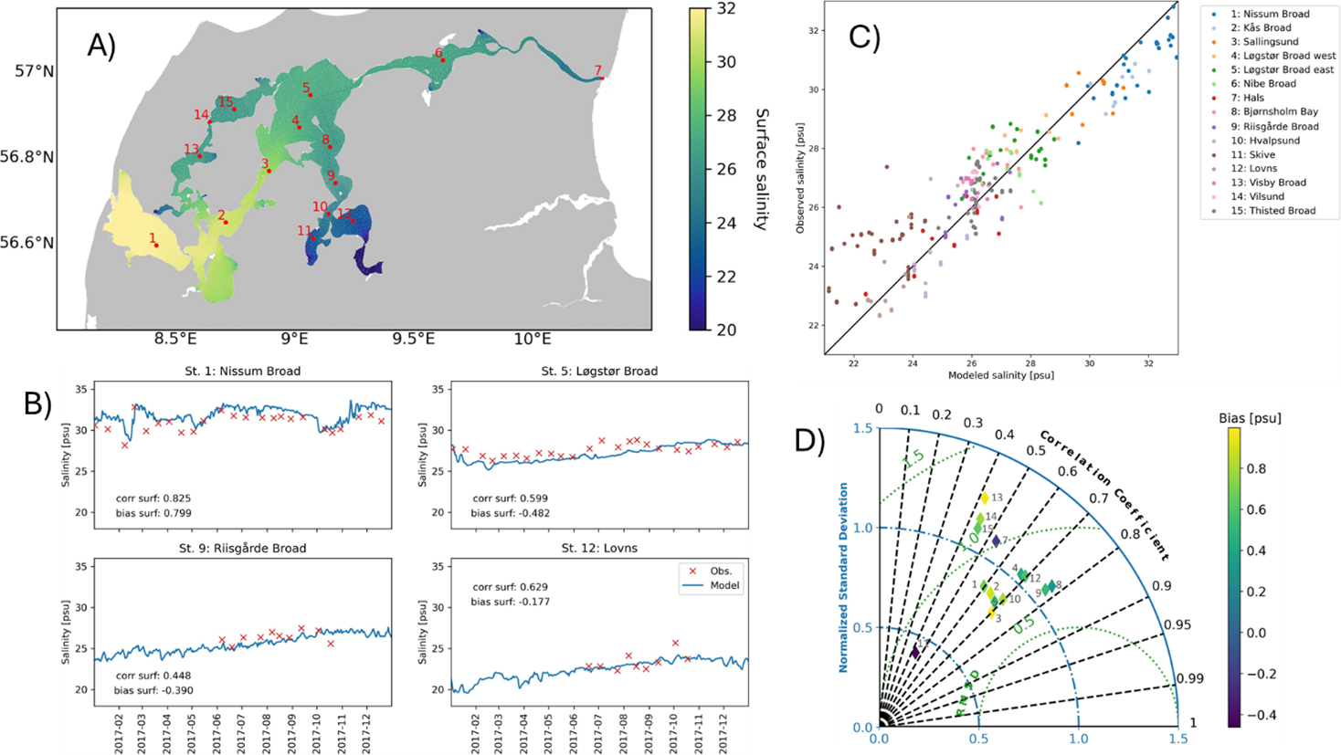
Figure 17. Salinity in Limfjorden. Modelled A) and measured B) values and model validation (C, D). A) Modelled average salinity, B) time series for selected stations in 2017, C) correlation between model and measurements for all stations, D) Taylor diagram showing correlation coefficient, bias (colour scale), and the normalized standard deviation between model and data. Compiled from Schourup-Kristensen et al. (2021).

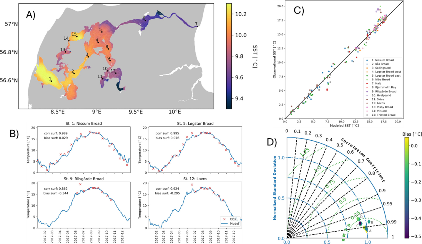
Figure 18. Temperature in Limfjorden. Modelled A) and measured B) values and model validation (C, D).  A) Modelled average salinity, B) time series for selected stations in 2017, C) correlation between model and measurements for all stations, D) Taylor diagram showing correlation coefficient, bias (colour scale), and the normalized standard deviation between model and data. Compiled from Schourup-Kristensen et al. (2021).

Climate scenarios for Limfjorden generally show the greatest change in physics for SSP5-8.5 and the latest period from 2090–2099 (Figs. 19 and 20). Salinity will decrease in all three scenarios by up to 2.2 psu in SSP5-8.5 due to greater runoff from land for the period 2090–2099 (Fig. 19). Water temperature will increase by 1–2 °C in SSP1-2.6 and SSP2-4.5, while it will rise by up to 5 °C in SSP5-8.5 in the last period (Fig. 20). The stratification of the water column is expressed by a PEA index, which indicates how much energy is required to mix it. A high index thus indicates strong stratification of the water column. In the most optimistic scenario, SSP1-2.6, there is only a small change in stratification in the future, while in the other two scenarios, stronger stratification is seen, especially in SSP5-8.5 for the last period (Figs. 19 and 20).

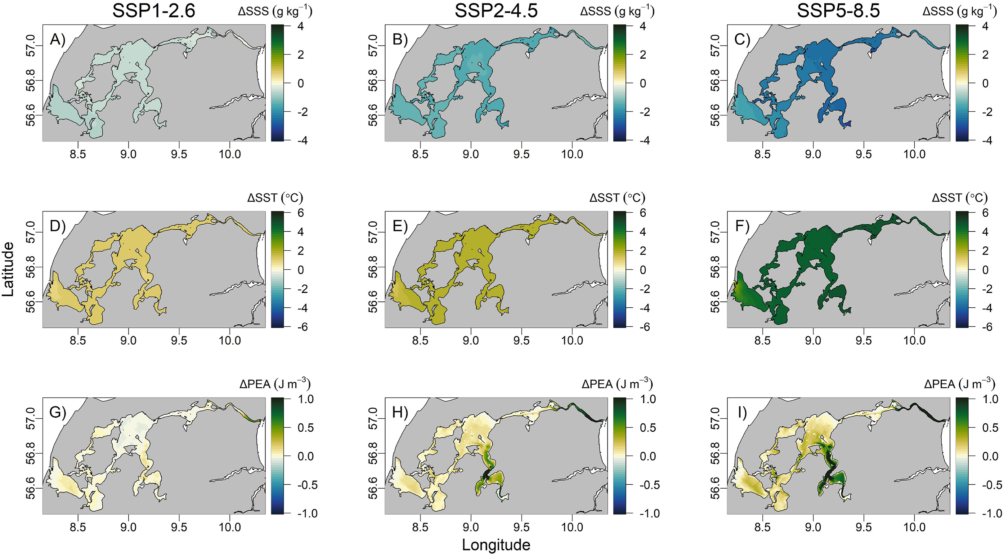
Figure 19. Changes in surface salinity (first row), surface temperature (second row), and stratification index (PEA, third row) in the three scenarios for the period 2090–2099 relative to the reference period. From Maar et al. (2024).

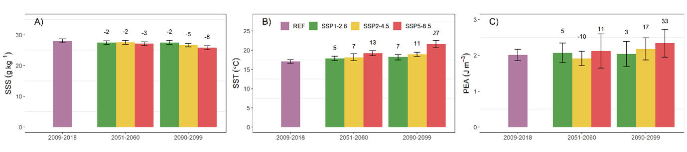
Figure 20. Average (±std) reference values (purple bar) and future changes in the three scenarios (green, yellow, red) for A) surface salinity (SSS), B) surface temperature (SST), and C) stratification Index (PEA) for the two time periods 2051–2060 and 2090–2099). Values above the bars are the percentage change relative to the reference period.

Results from the biogeochemical model during the reference period were compared with seasonal measurements from the ODA database. The seasonal variation of dissolved inorganic nutrients from the biogeochemical model during the reference period were compared with seasonal measurements from the ODA database. The seasonal variation of Dissolved Inorganic Nitrogen (DIN) is relatively large (Fig. 21A). In summer, the concentration is low at all stations, while the concentration increases during autumn and early winter. The model follows the seasonal cycle of the observations, although the model shows less short-term variation. Phosphate is also depleted in spring, but in mid-summer the surface concentration of phosphate increases again at all stations due to oxygen starvation-induced release from the sediment. The seasonal cycle of phosphate is well represented in the model, although there are occasionally higher summer values than seen in measurements (Fig. 21B).

The spring phytoplankton bloom, which takes place from February to April, is represented by the model in terms of timing and size (Fig. 21C). The subsequent low summer Chlorophyll a concentration and the autumn bloom in the Skive fjord are also represented in the model. During autumn and winter, the fjord has blooms of mixotrophic organisms in some years that are not represented by the functional plankton groups in the model.

The bottom oxygen concentration reaches a maximum in early spring when the water is mixed due to strong winds, the water temperature is low and biological consumption is reduced (Fig. 21D). After the spring bloom of phytoplankton and the accompanying transport of biological material to the sediment, the oxygen concentration decreases and reaches a minimum in late summer. The model reproduces the general trend of the seasonal cycle. However, the short-term variation is not fully represented by the model.

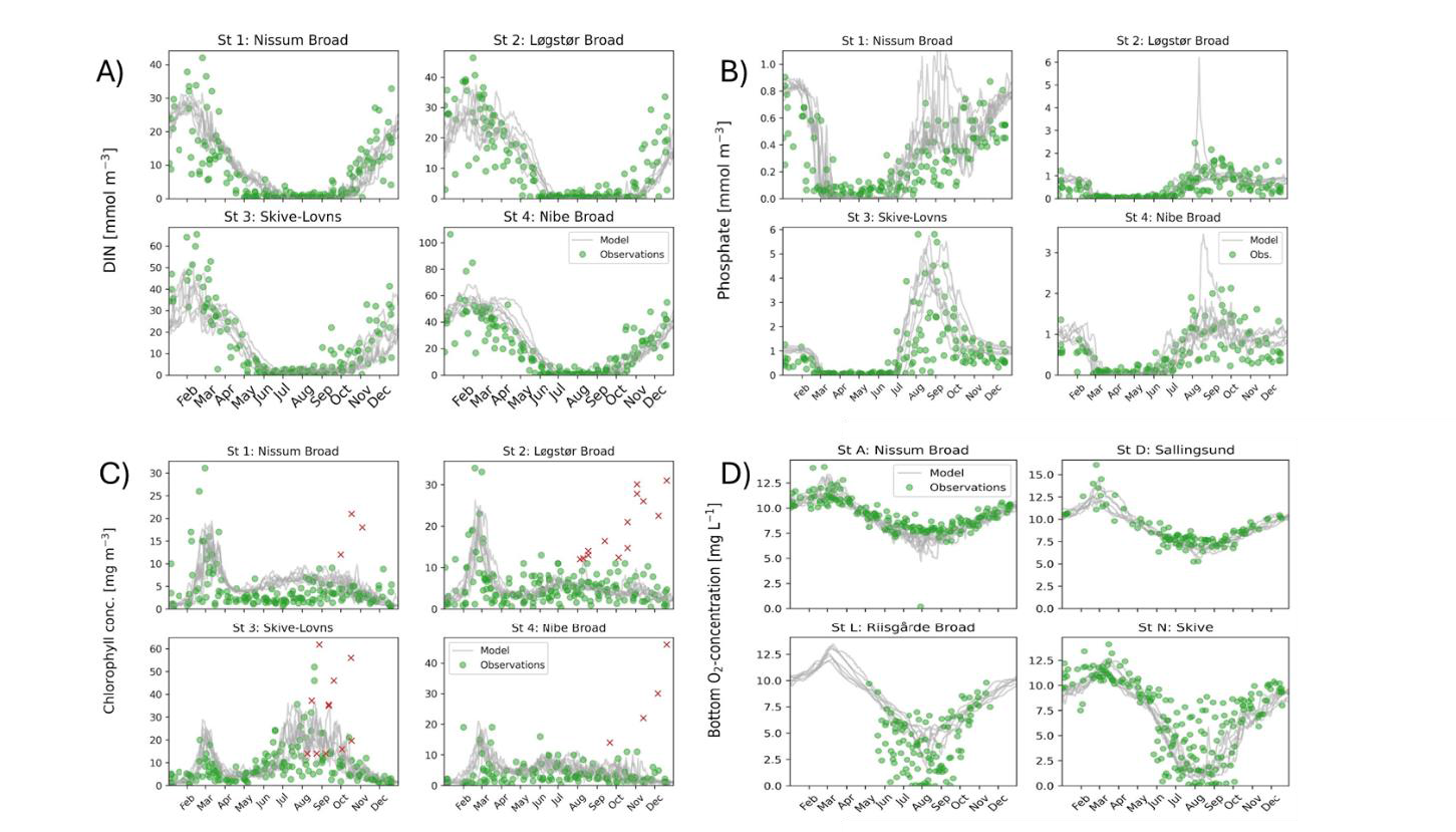
Figure 21. Comparison of model and measurements over time for A) DIN (NO₃+NH₄) concentration, B) phosphate concentration, C) Chl a concentration, and D) bottom oxygen concentration for the reference period for four selected stations. The grey lines are modelled values and the green circles measurements for each of the 10 years. The red crosses in C) are mixotrophic species not described in the model.

The model validation was also here summarised in Taylor plots for DIN, PO₄, Chl a and oxygen using the time series from 2011 to 2017. For closer examination of these plots, we refer to scientific papers by M. Maar and others, here a summary of the validation results. The modelled DIN has correlations higher than 0.80 at all stations, and nSD is within 1.00±0.25. The highest deviation is in the location Nibe Bredning, where the modelled values are on average underestimated. These errors are due to winter values, which are largely controlled by freshwater inflow. PO₄ has correlations around 0.70 at all stations. Phosphate concentration is overestimated (high nSD and deviation) at some stations in the model, possibly due to localised oxygen depletion in the model inducing a release of phosphate from the sediment.

The modelled Chl concentrations capture the seasonal cycle well with correlations around 0.50 except for Nibe Bredning due to minor short-term variability in the model in summer. Chl a is slightly overestimated at stations 1, 3 and 4 and nSD is within 1.00±0.25.

The statistics between modelled and observed oxygen concentration are best for stations with a full seasonal cycle of observations (St. A, B, C, I and N, F), while stations with only observed summer values have lower correlation and nSD due to the lack of seasonal variation in the model.

Climate scenarios for the Limfjord generally show greatest change in the ecosystem for SSP5-8.5 and the latest time period from 2090–2099 (Figs. 22 and 23). The greatest development of oxygen depletion is in the worst-case scenario SSP5-8.5, while there are no major changes in oxygen concentration for the less severe scenarios SSP1-2.6 and SSP2-4.5 (Figs. 22 A-C, Fig. 23B). Chl a concentration decreases slightly in the two lowest scenarios because the implementation of the Water Management Plans means that there is less nutrients available for algae growth (Figs. 22D-F). Overall, oxygen conditions and Chl a levels do not improve enough to achieve a better ecological status even with the implementation of the Water Management Plans (Fig. 23). This is because climate change in the form of increased temperature increases turnover and increased stratification prevents the supply of oxygen to the bottom water.

In the scenario SSP5-8.5, where the Water Management Plans nutrient reduction is not implemented, Chl a concentration is overall unchanged, but with a spatial redistribution (Fig. 23C). The biomass of benthic mussels is reduced <15% in the two optimistic scenarios due to lower food concentrations (Chl a), but the biomass is reduced more drastically (20–36%) in the worst-case scenario SSP5-8.5 due to the poorer oxygen conditions (Figs. 22 G-I, Fig. 23D).

The harvest of farmed mussels in the water column is expected to increase significantly in all scenarios as more mussel farms are established than in the reference period. Furthermore, farmed mussels are not significantly hampered by climate change induced oxygen depletion, as they are located at the top of the water column with good oxygen conditions and better access to food than at the bottom.

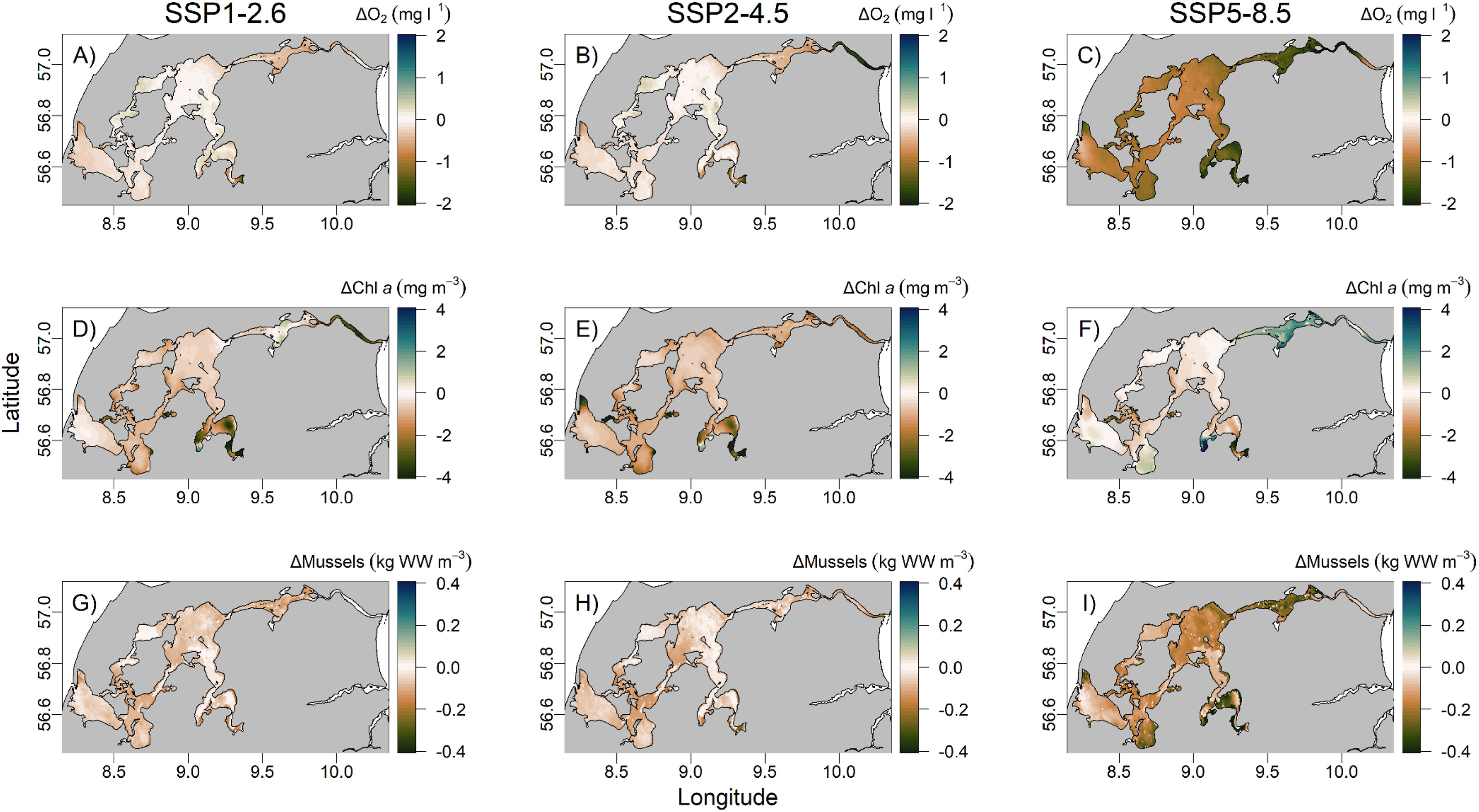
Figure 22. Changes in bottom oxygen (first row), surface Chl-a (second row) and mussel biomass (third row) in the three scenarios for the period 2090–2099. From Maar et al (2024).

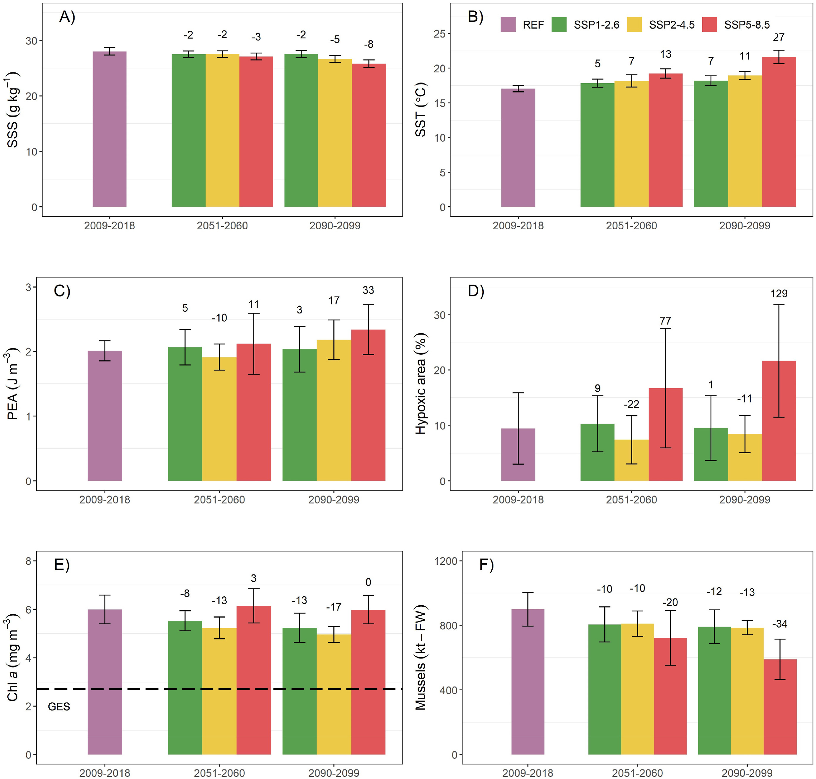
Figure 23. Summer (June to September) means (±SD) of A) sea surface salinity (SSS), B) sea surface temperature (SST), C) stratification index (PEA), D) hypoxic area (<4 mg l⁻¹) as percentage of total area, E) surface Chl a concentration, and F) benthic mussel biomass for the reference period (2009–2018) and the three scenarios and the two time-slices 2051–2060 and 2090–2099. The values above the columns are the percentage deviations from the reference period. The horizontal dashed line in E) indicates the thresholds for a good ecological status (GES).