3. Future scenarios for the North Sea and Baltic Sea

The downscaling of global earth system model climate projections to the North Sea and Baltic Sea was performed with the ocean model NEMO-SCOBI (Ruvalcaba-Baroni et al. 2024). The model has a regular grid with horizontal resolution of about 3.7 km and a vertical resolution of 3 m at the surface, decreasing to 22 m in the deepest parts of the domain (Norwegian trench). The Swedish Coastal Ocean and Biogeochemical model (SCOBI) is the biogeochemical component in NEMO-SCOBI (Ruvalcaba Baroni et al. 2024; Almroth-Rosell et al. 2015; Eilola et al. 2009). The SCOBI model includes 13 pelagic variables: dissolved oxygen, nitrate, ammonia, phosphate, mineral-bound inorganic phosphorus, dissolved silicate, three phytoplankton groups (diatoms, flagellates and others, and cyanobacteria), zooplankton and finally detritus pools of nitrogen, phosphorus and amorphous biogenic silica. The sediment includes four state variables of nitrogen, silicon, organic phosphorus and inorganic phosphorus. Hydrogen sulphide concentrations are represented by ’negative oxygen’ equivalents as described in Fonselius (1962).

Our regional downscalings are driven at the boundaries by the global climate model CNRM-CM6-1 (Voldoire et al. 2019). More specifically using its contribution to CMIP6 (O’Neill et al. 2016). The atmospheric forcing is not taken directly from the coarse global model, but instead first downscaled using the regional atmospheric model HCLIM (Belušić et al. 2020) to a horizontal resolution of 0.11 degrees to better capture local and regional winds and precipitation. These downscaled atmospheric runs are part of the EURO-Cordex project (Jacob et al. 2020) that provides regional atmospheric downscaling for Europe. The temporal resolution of our atmospheric forcing is hourly.

Three different scenarios were downscaled. The first is he historical period 1951–2014, where greenhouse gases, aerosols and other climate forcing parameters are kept close to those observed during the period. The two other scenarios are two different climate scenarios for the period 2015–2100, following two different shared socioeconomic pathways (SSPs), namely SSP1-2.6 and SSP3-7.0. SSP1-2.6 assumes a low emission, high mitigation future, while SSP3-7.0 corresponds to a high emission, low mitigation scenario. The number after the dash gives the radiative forcing in these runs in watts per m² compared to a preindustrial background. A higher value implies greater warming. 

Open boundary conditions for the ocean model are taken directly from the global climate model CNRM-CM6-1 for the respective scenarios. The variables used for forcing are salinity and temperature, sea surface height and barotropic currents. These variables were available only as monthly means, suggesting that high frequency variability at the boundaries will be muted in our simulations.

The daily runoff data from 1951 to 2100 was produced using dedicated CMIP6 simulations with the Hydrological Predictions for the Environment model, specifically the European application version 3.1.8 (E-HYPE; Donnelly et al. 2016), forced by the same climate model projections described above. These values were later modified by a factor of 0.88 after comparison with datasets from the North Sea (ICG-EMO database of European rivers; Lenhart et al. 2010) and from the Baltic Sea (Gustafsson et al. 2012), during the historical period of 1951–2014. The same scaling factor was assumed for the future period. A similar approach was used to estimate the nutrient loads from rivers, which include nitrate, ammonium, phosphate, silica and bioavailable detrital nitrogen and phosphate. For the historical period, E-HYPE nutrient loads (both CMIP6 scenarios) were yearly and basin wise adjusted, to the available observational data in the Baltic Sea (Gustafsson et al. 2012) and North Sea (ICG-EMO database of European rivers; Lenhart et al. 2010). Future river loads (after 2015) assume a constant scaling factor, which is the average of the yearly scaling factors computed between observations and E-HYPE model for a recent period (2006–2017). The method implies the underlying assumption of existing similar conditions of land use and E-HYPE performance in the recent period and in the future. As E-HYPE output does not include silica properties, future concentrations were obtained by assuming a climatology concentration computed for the historical period. The differences between the average for the historical reference period 1985–2014 (black) and the nutrient loads, runoff and river nutrient concentration are shown with time in Figs. 2 and 3. 

Atmospheric deposition for the historical period is based on a monthly data set at different basins of the Baltic Sea, provided by the Baltic NEST Institute (Savchuk et al. 2018). For the North Sea region, the study assumes that the nutrient atmosphere’s deposition is the same as in the Baltic Proper area. The data set was used directly as forcing in the historical period and used to compute a monthly climatology of the recent years (2006–2017) that was assumed for the future period. Details on the data sets and methods are also described in Ruvalcaba-Baroni et al. (2024).

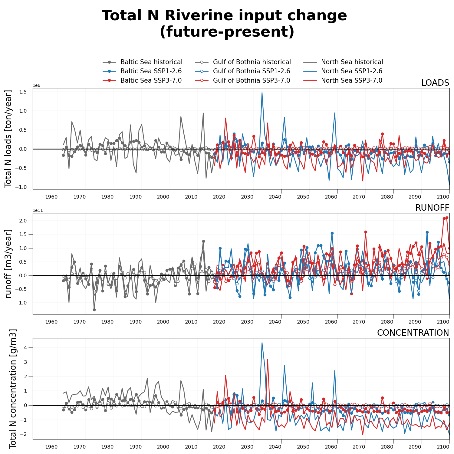
Figure 2. Nitrogen riverine input shown as regionally averaged time series of the differences between the historical period 1985–2014 (grey) and future developments with time. Development of nitrogen loads (top), runoff (middle) and river concentrations (bottom) with time for scenario SSP 1-2.6 (blue) and SSP3-7.0 (red) in the Baltic Sea (filled circles), Gulf of Bothnia (white circles), and North Sea (line).

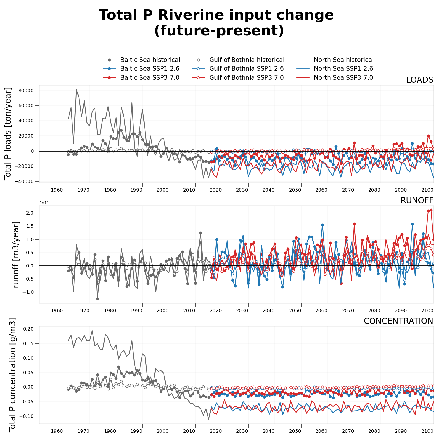
Figure 3. Phosphorus riverine input shown as regionally averaged time series of the differences between the historical period 1985–2014 (grey) and future developments with time. Development of nitrogen loads (top), runoff (middle) and river concentrations (bottom) with time for scenario SSP1-2.6 (blue) and SSP3-7.0 (red) in the Baltic Sea (filled circles), Gulf of Bothnia (white circles), and North Sea (line).

This section presents the downscaling of CMIP6 runs for one global model downscaled with one regional ocean model. These results add to the large ensemble of earlier CMIP3 and CMIP5 projections for the region, summarized, e.g., in the EN CLIME fact sheet Climate Change in the Baltic Sea (2021) for the Baltic Sea and in Quante and Colijn (2016) for the North Sea, and will be seen as a complement to those rather than independent results. The reason for this is the large variability in results and conclusions caused by natural variability as well as global and regional climate model uncertainties. These results should therefore be seen as the first step towards building a larger CMIP6 ensemble for the region.

For scenario SSP3-7.0, the surface temperatures increase with 2.5–3 °C in the Baltic Sea and 1–2 °C in the North Sea from the most recent 30-year period to the last 30-year period of the 21^st century (Fig. 4). For scenario SSP1-2.6 the increase is smaller with about 1 °C in the Baltic Sea and < 0.5 °C in the North Sea, and in some regions near the outer boundaries the temperatures decrease rather than increase. The changes are generally smaller in the bottom water than in the surface water, except for the decreasing temperatures in the North Sea that are larger in the bottom water than in the surface water. The changes in the Baltic Sea are within the range of changes reported earlier, e.g., Climate Change in the Baltic Sea (2021), considering that the CMIP6 reference period is later than those of the earlier CMIPs.

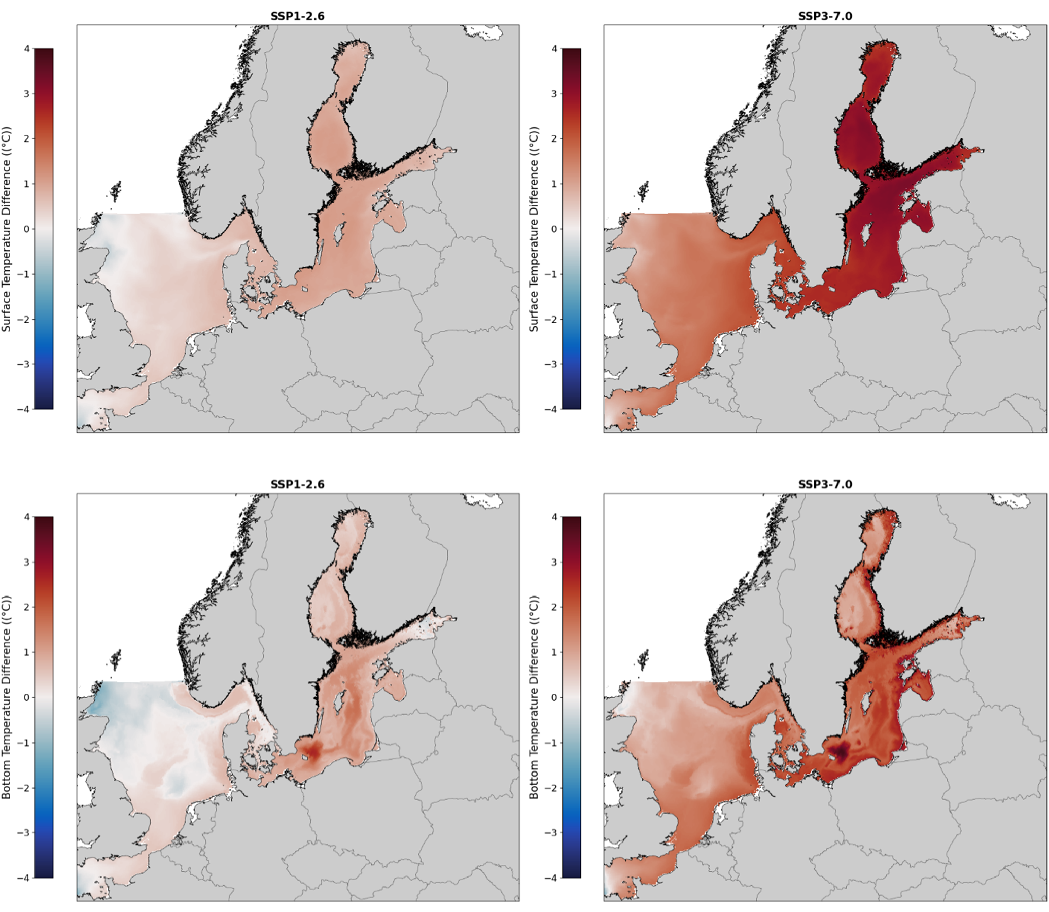
Figure 4. Surface (top row) and bottom (bottom row) temperature differences between the periods 1985–2014 and 2070–2099 for the scenarios SSP1-2.6 (left) and SSP3-7.0 (right).

The salinities show a general decrease (Fig. 5), most in the Baltic Sea bottom water with about 2 g/kg for the SSP3-7.0 scenario, and somewhat smaller decreases for the SSP1-2.6 scenario, Baltic surface waters and North Sea bottom and surface waters. In the central surface waters of the Skagerrak, there are increasing salinities, which are largest for the SSP1-2.6 scenario. This must be associated with a strengthening of the gradient between coastal and central Skagerrak salinities. Decreasing salinities are also found in earlier assessments for both the Baltic Sea (Climate Change in the Baltic Sea 2021) and North Sea (Quante and Colijn 2016). For the Baltic Sea, the results are sensitive to the assumption of no sea level rise, which would increase the salinities in the Baltic Sea due to larger inflows of saline water. The present result therefore probably represents an overestimate of the salinity decrease in the Baltic Sea.

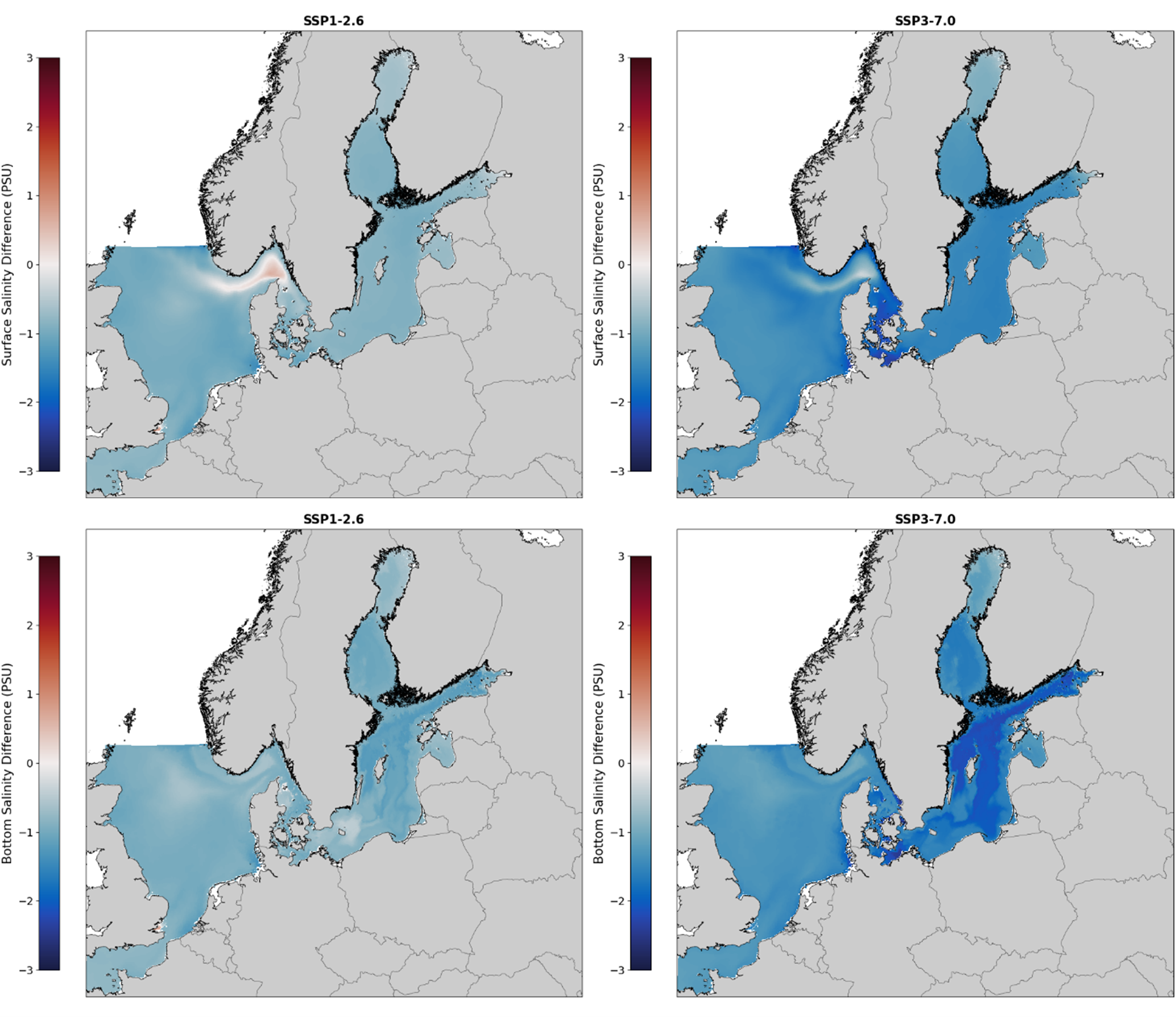
Figure 5. Surface (top row) and bottom (bottom row) salinity differences between the periods 1985–2014 and 2070–2099 for the scenarios SSP1-2.6 (left) and SSP3-7.0 (right).

The ice cover (Fig. 6) is decreasing for both scenarios, but most for SSP3-7.0, where ice will mainly be present only in the Gulf of Bothnia and Gulf of Finland, and where the central parts of the Bothnian sea will be ice free most years in the future period.

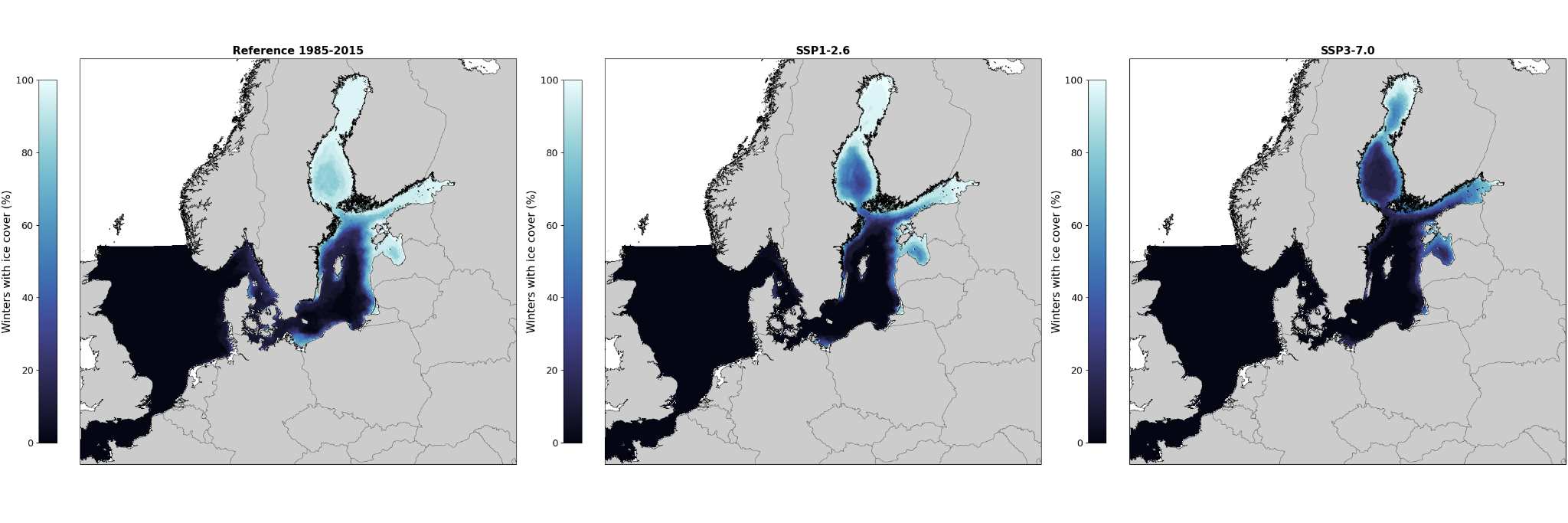
Figure 6. Percentage of winters with ice cover for historical period (1985–2014, left panel), and future period (2070–2099) for SSP1-2.6 (central panel), and SSP3-7.0 (right panel).

The time evolution of sea surface temperature and sea surface salinity for the North Sea, the Kattegat, and the Baltic Sea (Fig. 7) show the same changes as illustrated in Figs. 4 and 5, but they also show the multidecadal variability, which dominates the SSP1-2.6 signal for sea surface temperature, whereas the long-term climate trend is clearer in the SSP3-7.0 temperatures and for both scenarios for sea surface salinity. For sea surface temperature the increase is noticeably larger in the Baltic Sea than in the North Sea.

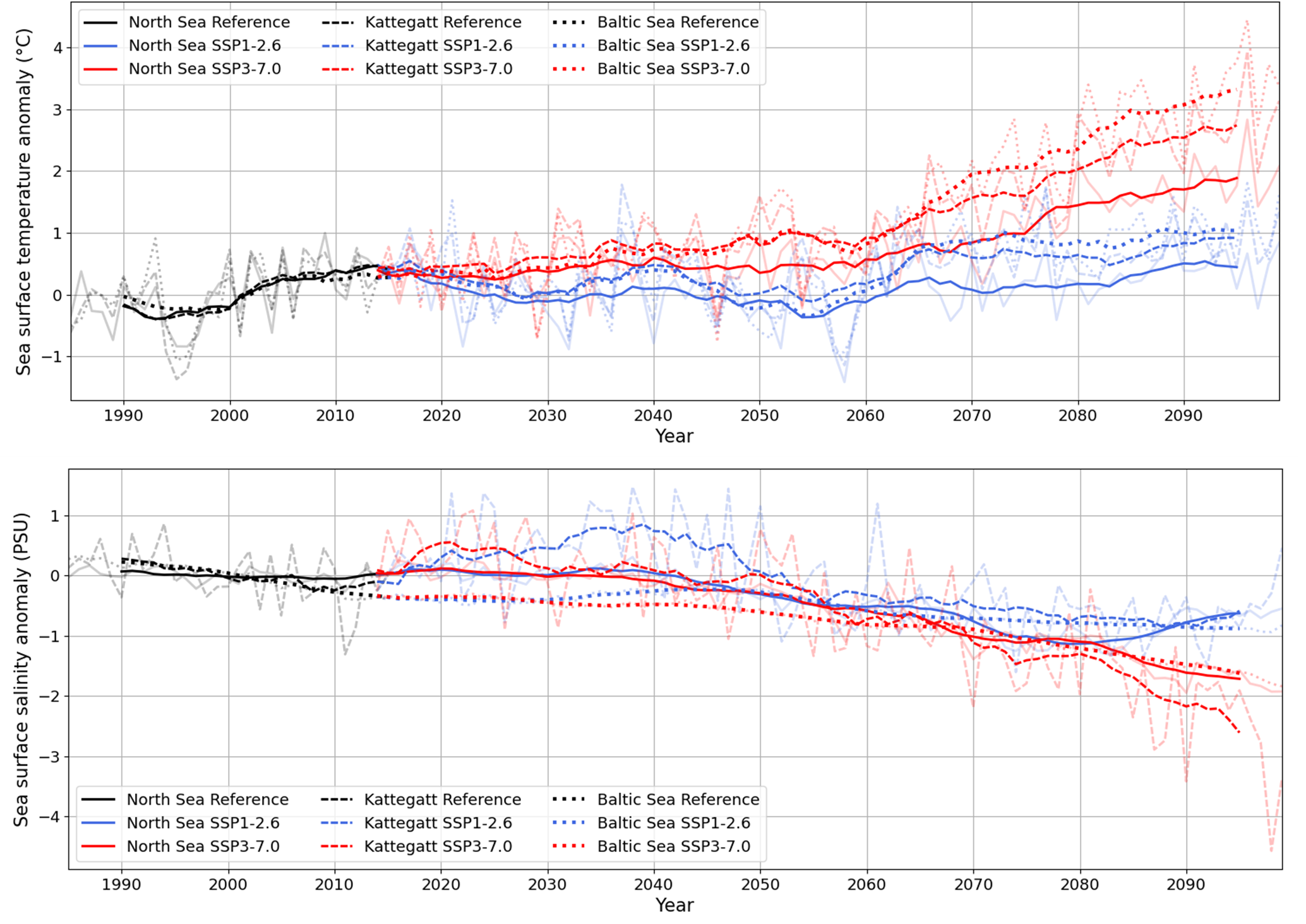
Figure 7. Sea surface temperature (upper panel) and sea surface salinity (lower panel) changes. Regionally averaged time series of the differences relative to the historical period 1985–2014 for the scenarios SSP1-2.6 (blue) and SSP3-7.0 (red) in the three regions North Sea (solid), Kattegat (dashed) and Baltic Sea (dotted). Transparent lines represent the annual mean, whereas the bold lines show a 10-year running mean.

The difference between the future (2070–2099) and historical period (1985–2014) surface average winter dissolved inorganic nitrogen (DIN), shows a decrease in a large part of the coastal areas in the Baltic Sea and North Sea. However, in the Gulf of Bothnia, along the Scotland coast, southern England and to a small extent also along the eastern coast of southern Sweden, DIN increases (Fig. 8, top). This pattern suggests a strong influence of the riverine nutrients input and consequently its main assumptions. In most areas, E-HYPE future adjusted projections indicate an increase in runoff and generally a decrease in nutrient loads and nutrient concentration (Figs. 2 and 3). Exceptions are the discharges in the Gulf of Bothnia (Figs. 2 and 3) and Scotland (not shown), where future river loads show a slight increase, where DIN increase is detected. As scenario SSP 3-7.0 projects a higher runoff increase, the pattern is enhanced and the winter DIN concentration differences between future and present are higher. Spatially, the changes in averaged winter DIN concentrations are relatively more important in the Kattegat (decrease) than in the North Sea (decrease) and in the Baltic Sea (increase), as shown in Fig. 8 (bottom) through the whole simulation period.  Similar results are found for winter dissolved inorganic phosphorus (DIP) concentrations (Fig. 9 bottom). There is a projected decrease in most of the Baltic Sea and coastal areas with some exceptions that likely result from the influence of the increased riverine phosphorus input, e.g. Gulf of Bothnia (shown in Fig. 3) and Gulf of Riga (not shown).

In general, the nutrient loads are projected to decrease in the future scenarios, with less decrease in the SSP3-7.0 scenario compared to the SSP1-2.6 scenario (or slight increase), which is also reflected in the nutrient concentration changes. Thus, the decrease in dissolved phosphate in the Kattegat area, the Baltic Sea and in the North Sea are larger in the SSP1-2.6 scenario (Fig. 9 top). The decreases are found along the southern North Sea coastline, the Kattegat area and the Baltic proper (Fig. 8 bottom). 

Changes in the riverine nutrient loads and runoff will imply changes in biogeochemical processes, namely in the primary production and phytoplankton concentration (Figs. 10 and 11), and ultimately in bottom oxygen conditions (Figs. 12 and 13). In a general view, the system is highly dominated by the riverine loads. In the above identified areas where nitrogen and phosphate concentrations were projected to decrease, chlorophyll concentrations are projected to be reduced (Figs. 10 and 11) and bottom oxygen concentrations to increase (Figs. 12 and 13).

In summary, the results show the importance of riverine nutrient loads in the Baltic Sea and North Sea biogeochemical variables dynamics. In general, the scenario SSP1-2.6 conditions project an overall improvement in water quality state and eutrophication conditions in the study area. Nutrient loads from rivers are reduced, primary production is reduced, and bottom oxygen conditions improve in most of the areas. Scenario SSP3-7.0, in turn, corresponds to a worse scenario by projecting less decreased riverine loads, but higher runoff, which leads to higher primary production and eutrophication processes in the system. However, this scenario does not seem to be worse than the current conditions and will even project an improvement of the ecosystem dynamics in terms of primary production and eutrophication problems. 

The results of the present study agree with previous studies conducted in the Baltic Sea area (Saraiva et al. 2019a, b) where conclusions indicate that for most of the included future scenarios (within the previous CMIP5 ensemble) the overall water quality state of the Baltic Sea is expected to improve, as long-lasting consequence of on-going nutrient load reductions since the 1980s. The impact of warming climate may amplify the effects of eutrophication and primary production. However, effects of changing climate, within the range of considered greenhouse gas emission scenarios, are smaller than effects of considered nutrient load changes. Generally, water quality conditions are expected to improve.

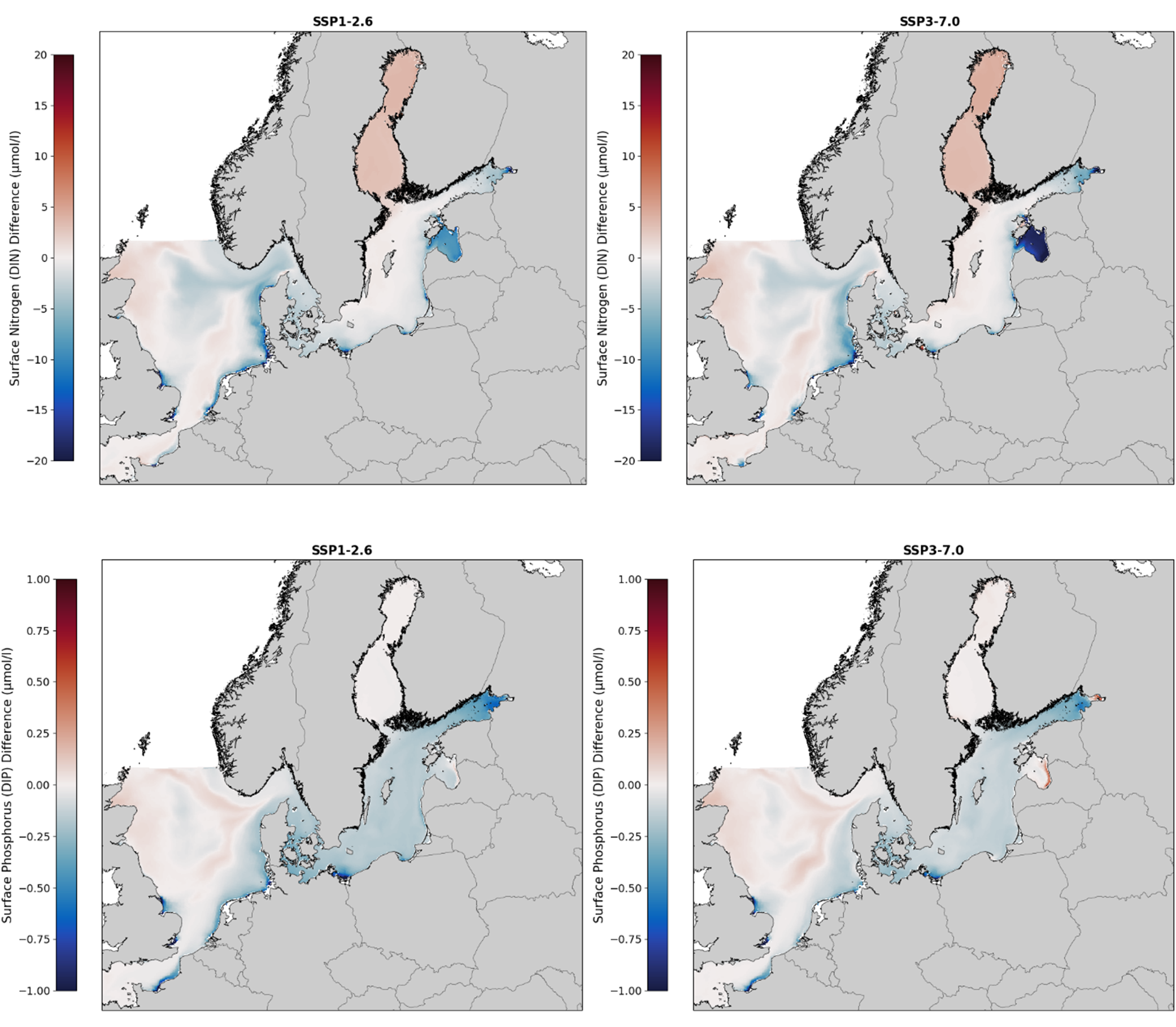
Figure 8. Winter surface Dissolved Inorganic Nitrogen concentration, DIN (top row) and winter Dissolved Inorganic Phosphorus concentration, DIP (bottom row):  differences between average present conditions (1985–2014) and future scenarios (2070–2099) SSP1-2.6 (left) and SSP3–7.0 (right).

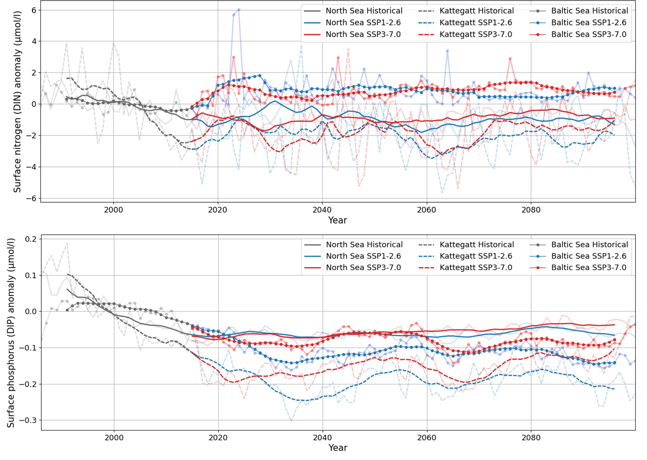
Figure 9. Winter dissolved inorganic nitrogen (DIN) (top bar) and dissolved inorganic phosphorus (DIP) concentration changes: Regionally averaged time series of the differences relative to the historical period 1985–2014 for the scenarios SSP1-2.6 (blue) and SSP3-7.0 (red) in the three regions North Sea (solid), Kattegat (dashed) and Baltic Sea (dotted). Transparent lines represent the annual mean, whereas the bold lines show a 10-year running mean.

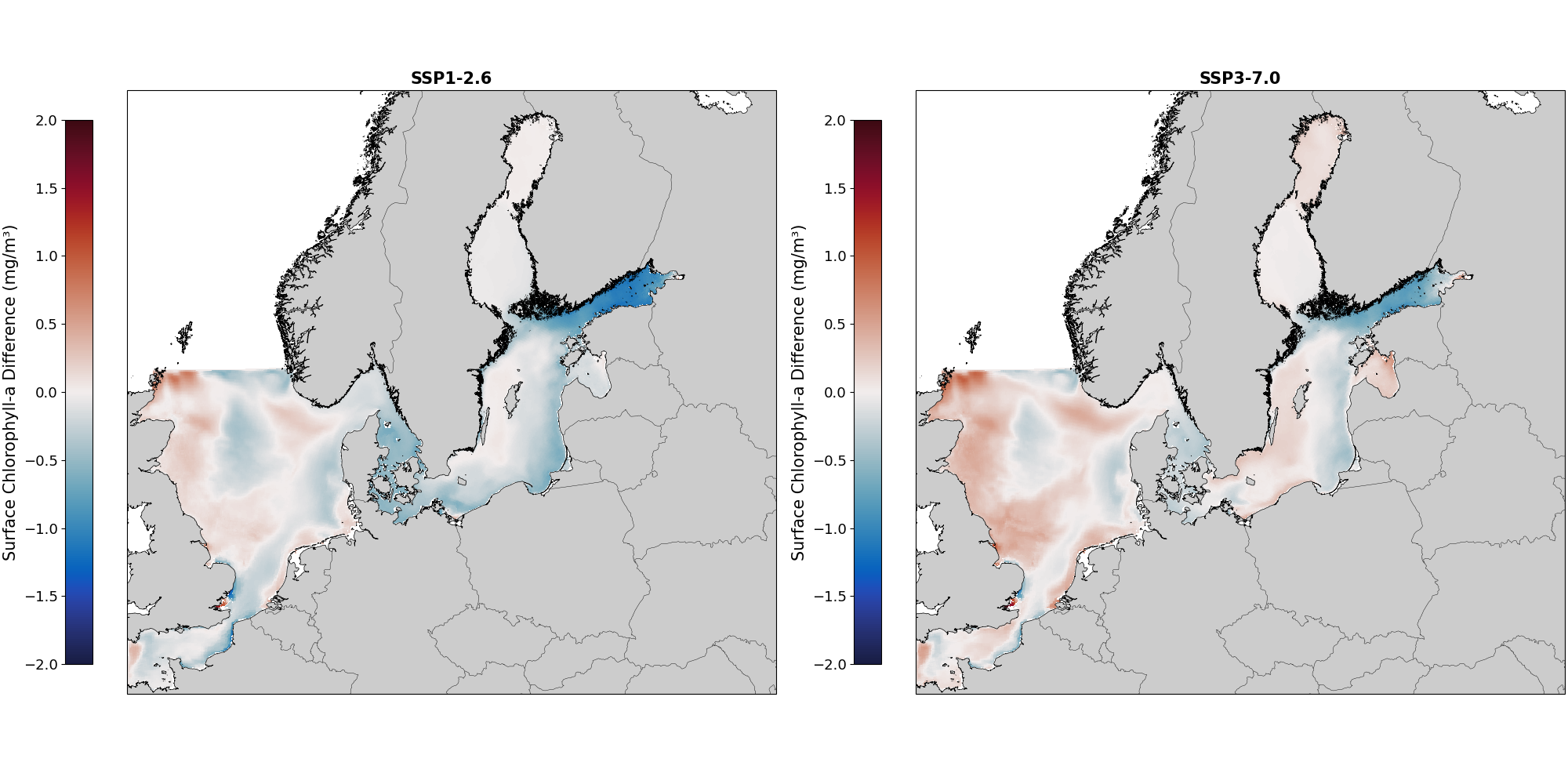
Figure 10. Surface chlorophyll-a concentration: differences between average current conditions (1985–2014) and future scenarios (2070–2099) SSP1-2.6 (left) and SSP3-7.0 (right).

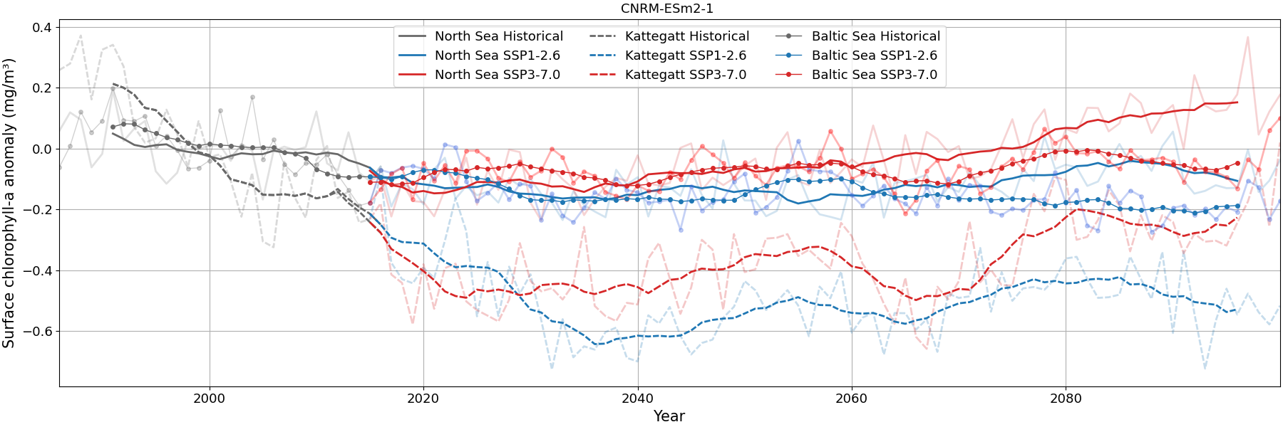
Figure 11. Surface chlorophyll-a concentration changes: Regionally averaged time series of the differences relative to the historical period 1985–2014 for the scenarios SSP1-2.6 (blue) and SSP3-7.0 (red) in the three regions North Sea (solid), Kattegat (dashed) and Baltic Sea (dotted). Transparent lines represent the annual mean, whereas the bold lines show a 10-year running mean.

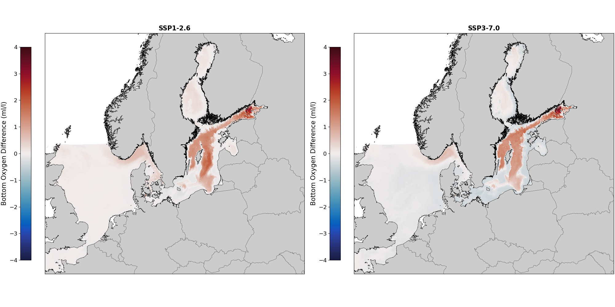
Figure 12. Bottom oxygen concentration: differences between the periods 1985–2014 and 2070–2099 for the scenarios SSP1-2.6 (left) and SSP3-7.0 (right).

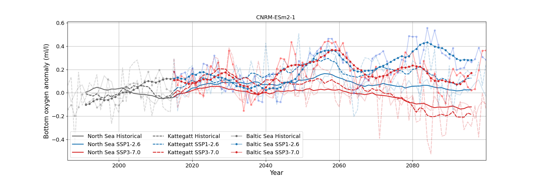
Figure 13. Bottom oxygen concentration changes: Regionally averaged time series of the differences relative to the historical period 1985–2014 for the scenarios SSP1-2.6 (blue) and SSP3-7.0 (red) in the three regions North Sea (solid), Kattegat (dashed) and Baltic Sea (dotted). Transparent lines represent the annual mean, whereas the bold lines show a 10-year running mean.