3. Methods
3.1 Method: Scaling of ecodesign savings from EU level to the Nordic countries
The method for calculating the ecodesign savings for each country by scaling down EU savings is quite simple. As shown in the equation below, country savings are calculated by multiplying the EU savings with a country- and product group-specific downscaling factor. All relevant scales, references, and specific assumptions appear in the notes on the scale-down module at Nordcrawl.org.
Country\,savings\,=\,EU\,savings\,*\,downscaling\,factor
3.1.1 Top-down: Choosing between scaling factors
When choosing a feasible scaling factor, the question to answer is the following: How much of the total EU savings does this country account for? In the following, I explain the factors that must be considered to answer this question.
First, we must examine the generic/basic equation for a scaling factor – the energy share – assuming that the savings are proportional to the energy consumption:
Scaling\,factor=\frac{Country\,consumption}{EU\,consumption}
where the consumption
It should be noted that the “consumption per appliances in stock” may not be the same for the EU stock as in the specific country. If the stock of appliances in a country is newer or more expensive it might use less energy than The EU average and vice versa.
This equation shows that the three factors to consider are the stock, usage, and consumption per appliance in the stock. In many cases, at least one of these factors is the same for the EU as for the specific country, and in that case, it should not be considered because it does not add additional information to the scaling.
The stock of products compared to EU/market penetration
The first question concerns a specific country’s share of the EU stock. For example, if a country accounts for 5% of the EU stock, and the usage of the product is the same in all countries, then the scaling factor should be 5% (0.05).
In many cases, we do not know the actual stock. Still, the stock and usage can be substituted with another factor, such as ‘number of houses’ (like all houses have one unit of this product) or economic factors such as ‘GDP’, ‘energy consumption’, or ‘electricity consumption’. For those cases, a scaling factor is chosen based on a substitute factor. For instance, transformers are correlated with electricity consumption.
Usage
If a product’s usage differs from the EU average, this should be reflected in the scaling factor. For example, the usage of heating products is higher in the Nordic countries than the EU average. This can be corrected by using heating degree days
Heating degree days (HDD) are a measure of how cold the temperature was on a given day or during a period of days.
Consumption per appliance in stock
The real question here is whether the appliances in one country are more efficient than the EU average and, if so, whether their greater efficiency is a result of EU policy or other factors. The ‘consumption per appliance in stock’ should only be considered when setting the scaling factor when other factors are known to cause the additional efficiency.
3.1.2 Data
EU savings
Data for the ecodesign savings comes from the 2023 EIA annual report, which VHK prepared for the European Commission. The report describes how the impact accounting is calculated as follows:
The projections in EIA are taken from the impact assessment reports, integrated with data from preparatory- and review-studies where necessary. These projections are the result of various years of study and have been discussed with stakeholders (see input-data verification above). They consider e.g. the historical and ongoing trends, the expectations from manufacturers, boundary conditions from EU policy, climate change effects, changes in EU population and households, trends in new-building and renovation, changes in user-demand (more comfort, larger displays and fridges, more light sources, rebound effects), and expected energy efficiency developments. Where the projection in the underlying studies does not cover the entire accounting period up to 2050, EIA extrapolates the existing trends without assuming any new measures, i.e. it is not in the scope of EIA to develop new policies. Projections use two scenarios:
- A ‘business-as-usual’ (BAU) scenario, which represents what was perceived to be the baseline without measures at the time of the (first) decision making, and
- An ECO scenario that is derived from the policy scenario in the studies which comes closest to the most recent measures taken, adapted to the final published regulation where necessary and possible.
- The differences in outcomes between the two scenarios are presented in EIA as ‘savings’ due to the policy measures. EIA takes into account product interactions, e.g. between ventilation units and space heating, the comments from the European Court of Auditors [12], and corrects for double counting in a transparent manner [13]. The EIA methodology is explained in detail in chapter 2 of the Status report.European Commission, Directorate-General for Energy, Ecodesign Impact AccountingOverview Report 2023 – Overview and status report, Publications Office of the European Union, 2024, (p. 11)
Scaling factor input
Input for the scaling factor highly depends on the data sources available for a specific country. The most common data sources are the following:
- Eurostat
- Odyssee-Mure database
- National statistics
- National report (such as a report on data centres in Norway)
- Stock calculated in the bottom-up model
- Stock from the EIA report
Source | Explanation |
Eurostat | Eurostat is the statistical office of the European Union. It provides data on population, energy, and electricity. |
Odyssee-Mure database | The Odyssee database concerns energy-efficiency indicators and energy consumption by end-use and underlying drivers in industry, transport, and buildings. The database provides consumption data for industry, residential, and service sectors. |
National statistics | National statistical offices. They provide national data that are not included in Eurostat or Odyssee. An example is Statistics Iceland, https://statice.is/ |
National reports | National reports provide specific input for the consumption of a particular product group in one country. An example is the Norwegian report Energibruk fra datasentre i Norge – NVE 2019 - Energiavdelingen - Jarand Hole og Hallgeir Horne http://publikasjoner.nve.no/faktaark/2019/faktaark2019_13.pdf |
Stock calculated in the bottom-up model | Stock calculation from the NordCrawl bottom-up model, which is described later in this report. One example is the stock of dishwashers in Finland. |
Stock from the EIA report | In the EIA report, the total EU stock is calculated. The stock is used, for example, for the scale for dishwashers in Finland. |
Survey | Survey of households conducted for this study. |
Table 1: Sources
Preferably, the data for the scaling should be from between 2010 and 2020.
3.1.3 Survey
To improve the accuracy of the downscaling factors used in the top-down model, a survey inspired by the Danish ElmodelBolig survey was conducted in households in Finland and Norway. This survey aimed to gather more representative data on heating, water heating, and ventilation systems in these countries. Denmark was not included because data from previous surveys already existed; Iceland was too small to include, and Sweden had another approach and data sources.
Nordstat administered the survey, targeting a representative sample of 1025 respondents in each country. The questionnaire, originally in English, was translated into the local languages to ensure better understanding and response quality. The survey covered background information and specific questions related to heating, water heating, and ventilation systems in households.
The results were weighted to ensure that they accurately represented the population in each country. The data collected from this survey provided valuable insights into the primary heating sources, water-heating methods, and the use of heat pumps for cooling during summer. This information was then used to refine the downscaling factors in the top-down model, leading to more precise estimations of energy savings from ecodesign and energy-labelling policies in the Nordic countries.
The table below presents a comparison of the survey results for Finland and Norway, data from Denmark from the Danish ElmodelBolig Survey, and data for Iceland obtained from other sources.
Table 2: Primary heating source in Nordic countries (excluding Sweden)
FI | NO | DK ElmodelBolig DK 2022, Elmodelbolig.dk | IS Sveinbjorn Bjornsson, Geothermal Development and Research in Iceland (Ed. Helga Bardadottir. Reykjavik: Gudjon O, 2006) | |
District heating | 47% | 9% | 49% | 90% |
Heat pump (air-air) | 7% | 26% | 6% | |
Heat pump (air-water) | 4% | 3% | 4% | |
Heat pump (exhaust air) | 1% | 1% | 0% | |
Heat pump (liquid-water/geothermal/bergvarm) | 8% | 2% | 2% | |
Central heating with boiler/furnace – oil | 4% | 1% | 2% | |
Central heating with boiler/furnace – wood pellets | 1% | 0% | 2% | |
Central heating with boiler/furnace – firewood /briquettes/straw | 2% | 0% | 2% | |
Central heating with boiler/furnace – gas | 0% | 0% | 12% | |
Central heating with boiler/furnace – electricity | 2% | 1% | 0% | |
Traditional electric radiators | 12% | 21% | 6% | 10% |
Electric heater with fan | 0% | 3% | 2% | |
Wood stove(s) | 2% | 17% | 13% | |
Open fireplace | 5% | 1% | 1% | |
Electric floor heating | 3% | 10% | 11% | |
Oil radiators (electric radiator with oil) | 1% | 2% | 1% | |
Solar thermal collector (produces heat, not solar cells/PV) | 0% | 1% | ||
Do not know | 4% | 3% |
Table 3: Primary water heating
FI | NO | DK ElmodelBolig DK 2022, Elmodelbolig.dk | IS Assumed based on: Sveinbjorn Bjornsson, Geothermal Development and Research in Iceland (Ed. Helga Bardadottir. Reykjavik: Gudjon O, 2006) | |
District heating | 46% | 9% | 59% | 90% |
Heat pump – hot water | 7% | 7% | ||
Central heating with boiler/furnace – oil | 5% | 2% | 2% | |
Central heating with boiler/furnace – wood pellets | 1% | 0% | 2% | |
Central heating with boiler/furnace – firewood/briquettes/straw | 2% | 0% | 2% | |
Central heating with boiler/furnace – gas | 0% | 1% | 12% | |
Electric water heater | 28% | 70% | 10% | 10% |
Solar thermal collector | 0% | 0% | 2% | |
Do not know | 11% | 11% |
3.1.4 Energy types
The model considers the following ‘types’ of energy:
- Primary energy
Primary energy is determined as follows: ‘
only electricity’ * primary energy factor for electricity + ‘only fuel’.
The primary energy factor for electricity was 2.5 and was adjusted to 2.1 in 2018 through the Energy Efficiency Directive (2018/2002). The primary energy factor can be changed for each country in the system.
- Only electricity
The savings in electricity.
- Only fuel
Savings in fuels such as oil, gas, and wood. - Final energy
The total savings in the final energy is 'only electricity' + 'only fuel'.
In some cases, it might be necessary to exclude ‘only electricity’ or ‘only fuel’ if there are no savings in the energy type in the country. For example, if the water is always heated by electricity and never by fuel, then ‘only fuel’ should be excluded.
3.2 Bottom-up method
The bottom-up models require sales data and the distribution of sales across energy classes. The model was used for product groups for which these data were available: refrigerator, refrigerator/freezer, freezer (chest), freezer (upright), washing machine, dishwasher, and tumble dryer.
3.2.1 Background
The bottom-up method is based on an Excel bottom-up model developed for Sweden and Denmark. The new model was developed as an online tool on the NordCrawl platform and is based on the old model's method, which was updated to accommodate all Nordic countries and new requirements, such as rescaling energy labels (in March 2021).
The bottom-up tool's methodological basis is the Danish bottom-up stock model ELMODEL – domestic (Fjordbak Larsen et al. 2003).
The tool's basic equation is as follows:
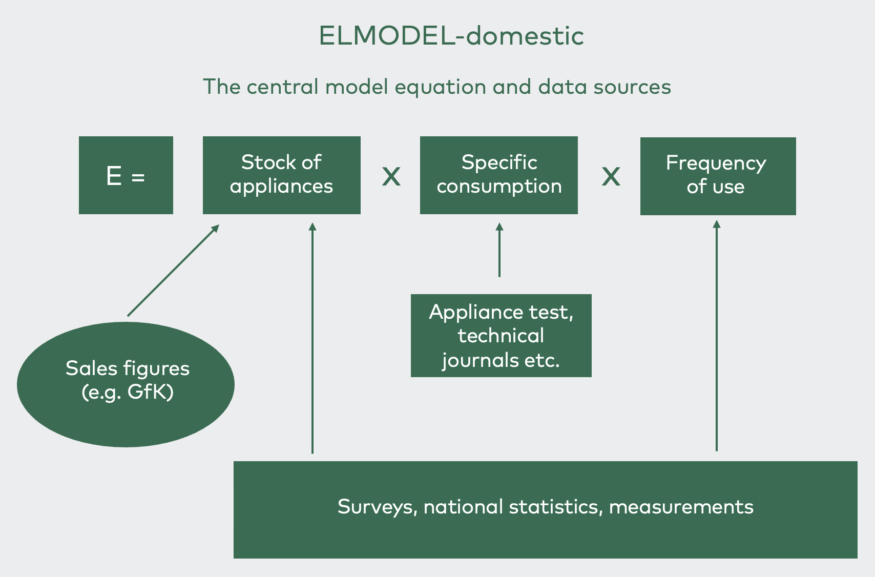
Figure 1: ElmodelBolig – domestic equation
The energy savings of the ecodesign and energy-labelling regulations were estimated by comparing the energy use of a product group in a baseline scenario (without regulations, or BAU) with the energy use of the product group in a policy scenario (with the effect of the regulations).
Figure 2: Example of baseline and scenario consumption
3.2.2 The two scenarios
Baseline scenario | Policy scenario | |
Policy (MEPS + energy label) | NO | YES |
Sales number (total number sold per year) | Same as sale until 2021; from 2022, 2021 + natural development | Same as baseline scenario |
Energy class sales distribution (before 2022) | Same as first year + natural development; annually, 2% of the sale in each class is moved up one class | Sales distribution |
Energy class sales distribution (after 2022) | Same as before 2022 | Sales distribution 2022 + energy label effect + ecodesign cut-off |
Rescaled label (2022) | NO | YES (dishwasher, washing machine, refrigeration) |
Table 4: Characteristics of the two scenarios
Ideally, the estimations would be based on data for the stock of appliances in the households by energy class, as shown in Figure 3. Detailed data of this kind are not collected in any Nordic country for any product groups. Attempts have been made to use surveys to collect this type of data in Denmark
ElmodelBolig
The next step in the model is to calculate a projection of the sales and the stock. For the baseline scenario, this is done as a simple forecast of the total sales (e.g., linear trend) and an assumed natural development in the sales distribution on energy classes.
With these inputs, the stock per energy class in a given year can be calculated as the sum of all sales until then that survived according to the lifespan distribution; see Figure 3. The figure illustrates how the lower energy classes are phased out, while the higher energy classes comprise larger shares of the stock.
A policy scenario parallel to the baseline scenario is used to estimate the effects of ecodesign (minimum energy performance standards [MEPS]), limiting the sales to the allowed energy-efficiency classes according to the legislation stages that successively come into effect. If a particular energy class is banned through an ecodesign MEPS criteria, the sales are simulated at the next energy class level. This is illustrated in Figure 3, where sales of banned energy classes are assumed to be zero in the years after the ecodesign requirements enter into force, which, in this example, occurs in two stages in 2022 and 2025.
The estimated savings caused by the ecodesign requirements (MEPS) are the difference between the baseline scenario curve and the policy scenario curve. Note that the natural development of the sales distribution remains active in the ecodesign scenario, preventing the ecodesign scheme from accounting fully for the efficiency improvements in sales.
The tool also provides a means to estimate the effects of energy labelling. This process is similar to natural development simulation, that is, setting an assumed annual change in percent towards more sales in higher energy classes. This shift in sales is illustrated in Figure 3. The energy labelling affects the sales in all energy classes every year. The effects of labelling are calculated in parallel to the ecodesign effects, ensuring that any effect in sales that MEPS already simulates are not accounted for when simulating the effects of labelling. This also ensures that no measures are double counted.
Class | 2022 | 2023 | 2024 | 2025 | 2026 | 2027 |
G | 0 | 0 | 0 | 0 | 0 | 0 |
F | 44,370 | 43,917 | 43,469 | 0 | 0 | |
E | 65,929 | 66,153 | 66,365 | 109,592 | 109,343 | 109,088 |
D | 65,929 | 66,588 | 67,245 | 67,900 | 68,552 | 69,201 |
C | 2,684 | 3,988 | 5,292 | 6,597 | 7,901 | 9,205 |
B | 0 | 54 | 134 | 240 | 371 | 526 |
A | 0 | 0 | 1 | 4 | 9 | 16 |
Table 5: Example of banned energy class
* Class "F" banned
As mentioned above, the savings from the ecodesign and energy-labelling regulations are estimated as the difference between the base-case scenario and the policy scenarios for ecodesign and energy labelling.
3.2.3. Assumptions
Changeable assumption | Example | Explanation |
Start year data | 1995 | First year in the data series |
Starting year for baseline projections | 1996 | The first year where the baseline is projected; in most cases, the year after the times series starts |
Starting year for projections | 2023 | The first year of projections in the policy scenario. The starting years can be changed to focus on the policy effects for a shorter period |
End year for projections | 2050 | The last year in the projection and thus the last year in the analysis |
End year for sale | 2022/2050 | The last year of sales of this product group. 2021 was chosen for cases in which a new time series for the new label will replace the old label |
End year for baseline sale | 2050 | The last year of sale for the baseline |
Baseline development (% p.a.) | 2% p.a. | The natural development of the baseline; this assumes that energy efficiency will improve naturally without policies |
Lifetime | 12 years | The lifespan of a product |
EEI ref consumption | 380.7 kWh/year | The Energy Efficiency Index reference consumption calculated the equation in the regulation using assumed size(s) |
EEI ref size | 7 kg | The Energy Efficiency Index reference size(s) used for the consumption calculation |
Table 6: Table with assumptions (washing machine example)
The modelling is based on several other assumptions, including the following:
- A normally distributed lifetime of products typically has mean value between 8–16 years for white goods.
- The energy consumption per year reference was calculated using an assumed average size (or sizes) and the equations for the annual consumption per unit from the regulations. Some cases, such as that of refrigerators, have many options for different compartment types, etc. In those cases, we simplified the product to the most common types where data are available.
- Each energy class can be characterised by a mean annual energy consumption value. For example, on the old label for washing machines, class A++ has an EEI between 46 and 52, and the mean is EEI 49.
- The baseline is defined by a natural development in the market, which is 2% per year of the sales in the specific energy class are assumed to move one energy-efficient class up. This number can be adjusted because the market's development can differ for different types of products.
- Non-compliant sales, (below MEPS) move the sale to the nearest available energy class.
- The effect of labelling is simulated by shifting X% of the sale in each energy class to the next most efficient labelling class every year, where X is assumed to be high (~25%) for the first several years after the requirements come into force, after which it is lower (~5%). This assumption is based on knowledge from the introduction of energy labelling for white goods in the late 90s.
All assumptions can be modified for each simulated product group.
3.2.4 Data
The following data sources were used for the modelling:
- Sales data from APPLiA Danmark and Sweden (the Association for Suppliers of Electrical Domestic Appliances); the association collects sales figures for white goods from its members
- Elektronikkbransjen Norge, the Consumer Electronics Trade Foundation; members are suppliers, dealer chains, independent dealers, and workshops
- National energy statistics
- ElmodelBolig, a bi-annual Danish survey of about 2,000 households performed by Energistyrelsen
- Other product-specific reports, such as JRC for data centres; see footnotes
- NordCrawl
3.2.5 Data-sharing and sales-scaling
The sales data used to estimate the savings from ecodesign and the energy labelling of white goods are from APPLiA in Demark and Sweden (for only select years); this group collects sales data for white goods from their members. Likewise, Elektronikkbransjen in Norway collects sales data (the number of products and energy classes) from their members. It has been assumed that the Nordic consumers have approximately the same energy-efficiency preferences when buying white goods, which means that we can use the sales distribution of energy classes from Denmark, Norway, or Sweden in Iceland and Finland. The country that is the best match can be determined by examining factors such as housing type distribution and the economy. An argument for this assumption is the fact that online shops such as Elgiganten (known as Elkjøp Norway, Gigantti Finland) have similar websites and selections. The sales figures (the number of models sold per year) were scaled to adjust to different household stock. Sales data from Norway and Sweden cover fewer years than data from Denmark, so Danish sales data were used to extend those time series.
Country | Data source | Scaling factor (for the annual sale in units of appliances) |
Denmark | 1995–2022: APPLiA DK | – |
Sweden | 1995–2016: APPLiA DK, 2017–2022: APPLiA SE + 2022 DK dist | SE sales/DK sales (per product group) |
Norway | 1995–2005: APPLiA DK, 2006–2022: Elektronikkbransjen Norge | NO sales/DK sales (per product group) |
Finland | 1995–2022: APPLiA DK | FI households/DK households |
Iceland | 1995–2022: APPLiA DK | IS households/DK households |
Table 7: Sales data-sharing and data-scaling
Rescaled energy labels
During the last project, the energy labels for the appliances in this project were rescaled. The rescaling came into force on 1 March 2021. Therefore, no sales data for the new, rescaled energy class distributions were available at that time, and we thus had to create a conversion from the old energy label to the new. For this project, sales data for the new energy label are available, so we did not have to convert them.
At the same time, new, more stringent MEPS were introduced. To handle the new MEPS and the new label with the new thresholds for the energy-labelling classes, we decided to treat appliances with a new label as a new product, replacing the models with the old label. When calculating the savings, we added the savings from the old label to the savings from the new one. Over time, appliances with the old label will be replaced with appliances with the new label in the stock. The figure below shows how appliances with the new label replace those with the old label over time.
Figure 4: Example of how the stock changes from the old to the new energy label
3.2.6 Uncertainty
The bottom-up modelling is data demanding, and the quality of the results naturally depends on the quality of the input data; especially detailed sales data can improve the quality. Since these data can be difficult to obtain, assumptions must be introduced to establish sales data at the needed granularity, which adds to the uncertainty.
The long-term projections of the model are also uncertain, since many of the assumptions made to establish the bottom-up basis are not valid over a long period. The model should only be used for projections of five to 15 years, which is equal to one generation of most white goods. Otherwise, the model should be developed further to incorporate top-down elements to guide some assumed developments (or statistics). An example of long-term uncertainty in a bottom-up model is that it is difficult to predict when a new technology is introduced for an appliance (often called technology leaps; e.g., the use of heap pumps in tumble dryers). Another example is consumer preference changes. In some Nordic countries, we observed a change from chest freezers to upright freezers. If the model is used to project too far into the future, such changes will not be adequately reflected.
In summary, the model can estimate the composition of the stock in any given year in terms of energy parameters using data for how the actual annual sales are distributed over energy classes. This enables us to calculate the total energy consumption for a baseline situation, as well as the energy consumption for policy scenarios. The difference between the baseline scenario and the policy scenario constitutes the savings at the national level that is attributable to the policies.
3.2.7 Quality assurance of assumptions
The following quality controls were performed to ensure the robustness of the assumptions.
Product penetration
We analysed the product penetration, which is the quantity of a product in a household (stock/households). Surveys in Denmark and Norway clarify the approximate expected penetration, and by comparing the calculated with the expected penetration, we can evaluate the assumptions. For example, the general penetration of a refrigerator is around one refrigerator per household. If the calculated penetration is 0.5 refrigerators per household, there could be a problem with the scaling of sales data (in most cases, the Danish APPLiA data) or the assumed lifetime.
Comparison between countries
We compared the assumptions and results between Nordic countries. Some variations are expected due to different lifestyles, such as the popularity of dryers or housing types; many apartments have fewer washing machines and have shared washing machines, typically in the basement. However, the central assumption is that the results should be comparable, and we should be able to explain the variations logically.
3.3 Combining scale-down and bottom-up results
For product groups where bottom-up results are available, they are preferable to those from the scale-down method, as the bottom-up approach provides more accurate estimates. In these cases, rather than applying a scale-down factor to the EU savings, we directly replaced the EU savings with the country-specific savings calculated using the bottom-up method. This effectively meant using a scale-down factor of 100% for these product groups.
In Sweden, some savings for heating products were also calculated separately, and the results were added in the same way as for the bottom-up results. This further enhances the accuracy of the savings estimates for these specific product groups in Sweden.
This approach allowed us to combine the two methods into one comprehensive result, ensuring that we used the most accurate data available for each product group. By prioritising the bottom-up results where possible, incorporating separately calculated savings for certain product groups in Sweden, and relying on the scale-down method for product groups without detailed data, we generated a more precise overall estimate of the energy savings from ecodesign and energy-labelling policies in the Nordic countries.