Appendix for Chapter 2: An evaluation of fish stocks lacking quantitative assessments in Skagerrak

Supplementary Section 1: Species

Table S1: Species with a quantitative stock assessment relevant to the Skagerrak area.

Aphia ID	Species	Family	ICES_ID	ICES_Category	Hauls_NOSS	Hauls_NS-IBTS	Hauls_Total
126417	Clupea harengus	Clupeidae	her.27.3a47d,her.27.20-24	1,1.2	12294	77728	90022
126436	Gadus morhua	Gadidae	cod.27.47d20	1	4210	61012	65222
126444	Trisopterus esmarkii	Gadidae	nop.27.3a4	1	33687	23780	57467
126437	Melanogrammus aeglefinus	Gadidae	had.27.46a20	1	13580	35540	49120
127143	Pleuronectes platessa	Pleuronectidae	ple.27.420	1	1237	35372	36609
127136	Glyptocephalus cynoglossus	Pleuronectidae	wit.27.3a47d	1	5228	10872	16100
126441	Pollachius virens	Gadidae	pok.27.3a46	1	5361	6864	12225
126484	Merluccius merluccius	Merlucciidae	hke.27.3a46-8abd	1	3690	7948	11638
127160	Solea solea	Soleidae	sol.27.20-24	1	5	3744	3749
127149	Scophthalmus maximus	Scophthalmidae	tur.27.3a	2.1	1	424	425

Table S2: Eighty-two species observed in the two surveys in the Skagerrak area. The “x” in column “L” indicates for which species species-specific landings are available. Similarly, the “x” in column “S” indicates for which species, a reliable (CV < 1.5) relative abundance index could be estimated.

Aphia ID	Species	Family	ICES ID	ICES Stock cat	# NOSS	# NS-IBTS	# total	Shape	Habitat	Gear group	L	S
126438	Merlangius merlangus	Gadidae	whg.27.3a	3.23	11547	65044	76591	fusiform/normal	near-bottom	6	x	x
127137	Hippoglossoides platessoides	Pleuronectidae			15111	54192	69303	short and/or deep	bottom	4	x	x
127139	Limanda limanda	Pleuronectidae	dab.27.3a4	3.22	274	35652	35926	short and/or deep	bottom	4	x	x
150637	Eutrigla gurnardus	Triglidae	gug.27.3a47d	3.23	474	18084	18558	elongated	bottom	2	x	x
126450	Enchelyopus cimbrius	Lotidae			1722	11352	13074	elongated	bottom	2		x
126446	Trisopterus minutus	Gadidae			1523	10476	11999	fusiform/normal	near-bottom	6		x
127140	Microstomus kitt	Pleuronectidae	lem.27.3a47d	3.22	221	9048	9269	short and/or deep	bottom	4	x	x
127312	Maurolicus muelleri	Sternoptychidae			6156	2824	8980	elongated	near-bottom	5		x
105824	Chimaera monstrosa	Chimaeridae			7278	1224	8502	elongated	bottom	2	x	x
127118	Lycodes vahlii	Zoarcidae			0	7792	7792	eel-like	bottom	1		x
127141	Platichthys flesus	Pleuronectidae	fle.27.3a4	3.2	4	7676	7680	short and/or deep	bottom	4	x	x
154675	Lumpenus lampretaeformis	Stichaeidae			18	6716	6734	eel-like	bottom	1		x
126793	Callionymus maculatus	Callionymidae			32	6276	6308	elongated	bottom	2		x
126792	Callionymus lyra	Callionymidae			32	6040	6072	elongated	bottom	2		x
126439	Micromesistius poutassou	Gadidae			4712	476	5188	elongated	near-bottom	5
126715	Argentina silus	Argentinidae	aru.27.123a4	3.2	4964	156	5120	elongated	near-bottom	5
127214	Cyclopterus lumpus	Cyclopteridae			222	4440	4662	short and/or deep	near-bottom	7	x	x
158960	Coryphaenoides rupestris	Macrouridae	rng.27.3a	3.23	3983	20	4003	elongated	near-bottom	5	x	x
274100	Lycodes gracilis	Zoarcidae			1526	672	2198	elongated	bottom	2		x
126716	Argentina sphyraena	Argentinidae			35	1868	1903	elongated	bottom	2		x
127126	Arnoglossus laterna	Bothidae			0	1448	1448	fusiform/normal	bottom	3		x
127150	Scophthalmus rhombus	Scophthalmidae	bll.27.3a47de	3.22	0	1176	1176	short and/or deep	bottom	4	x	x
126440	Pollachius pollachius	Gadidae	pol.27.3a4	5.2	79	892	971	fusiform/normal	near-bottom	6	x	x
127379	Entelurus aequoreus	Syngnathidae			7	944	951	eel-like	bottom	1
127101	Lycenchelys sarsii	Zoarcidae			125	752	877	eel-like	bottom	1
126555	Lophius piscatorius	Lophiidae	anf.27.3a46	3.21	184	668	852	short and/or deep	bottom	4	x	x
127153	Buglossidium luteum	Soleidae			0	752	752	short and/or deep	bottom	4		x
126461	Molva molva	Lotidae			159	412	571	elongated	bottom	2	x	x
127082	Trachinus draco	Trachinidae			4	500	504	fusiform/normal	bottom	3		x
127251	Helicolenus dactylopterus	Sebastidae			444	56	500	fusiform/normal	bottom	3		x
127190	Agonus cataphractus	Agonidae			7	472	479	fusiform/normal	bottom	3		x
126904	Lesueurigobius friesii	Gobiidae			0	432	432	fusiform/normal	bottom	3		x
127255	Sebastes viviparus	Sebastidae			364	28	392	short and/or deep	bottom	4		x
126758	Anarhichas lupus	Anarhichadidae			3	364	367	elongated	bottom	2	x	x
126986	Mullus surmuletus	Mullidae	mur.27.3a47d	5	87	244	331	fusiform/normal	bottom	3
126756	Hyperoplus lanceolatus	Ammodytidae			0	324	324	elongated	bottom	2		x
126928	Pomatoschistus minutus	Gobiidae			0	288	288	fusiform/normal	bottom	3
126505	Gasterosteus aculeatus	Gasterosteidae			76	180	256	fusiform/normal	near-bottom	6
127203	Myoxocephalus scorpius	Cottidae			3	212	215	fusiform/normal	bottom	3		x
293018	Zeugopterus norvegicus	Scophthalmidae			10	160	170	short and/or deep	near-bottom	7		x
127389	Syngnathus rostellatus	Syngnathidae			0	160	160	eel-like	bottom	1		x
127138	Hippoglossus hippoglossus	Pleuronectidae			35	124	159	fusiform/normal	bottom	3	x	x
127387	Syngnathus acus	Syngnathidae			0	124	124	eel-like	bottom	1
126751	Ammodytes marinus	Ammodytidae			8	108	116	elongated	near-bottom	5
126501	Phycis blennoides	Phycidae			90	24	114	fusiform/normal	near-bottom	6	x	x
127427	Zeus faber	Zeidae			3	80	83	short and/or deep	near-bottom	7	x	x
127262	Chelidonichthys lucerna	Triglidae			0	80	80	elongated	bottom	2		x
126996	Pholis gunnellus	Pholidae			0	72	72	eel-like	bottom	1
127072	Leptoclinus maculatus	Stichaeidae			7	64	71	elongated	bottom	2
126448	Ciliata mustela	Lotidae			0	60	60	elongated	bottom	2		x
126281	Anguilla anguilla	Anguillidae			5	48	53	eel-like	bottom	1
126445	Trisopterus luscus	Gadidae			0	52	52	fusiform/normal	near-bottom	6		x
127393	Syngnathus typhle	Syngnathidae			0	48	48	eel-like	bottom	1
126795	Callionymus reticulatus	Callionymidae			8	28	36	elongated	bottom	2		x
126929	Pomatoschistus norvegicus	Gobiidae			32	4	36	fusiform/normal	bottom	3		x
150630	Echiichthys vipera	Trachinidae			1	32	33	elongated	bottom	2
293624	Liparis liparis	Liparidae			0	32	32	elongated	bottom	2		x
126752	Ammodytes tobianus	Ammodytidae			7	24	31	elongated	bottom	2
126447	Brosme brosme	Lotidae	usk.27.3a45b6a7-912b	3.2	29	0	29	elongated	bottom	2	x	x
127205	Triglops murrayi	Cottidae			1	28	29	elongated	bottom	2
126459	Molva dypterygia	Lotidae			23	4	27	elongated	bottom	2	x	x
126975	Dicentrarchus labrax	Moronidae			0	20	20	fusiform/normal	bottom	3
127146	Lepidorhombus whiffiagonis	Scophthalmidae			1	16	17	fusiform/normal	bottom	3
126442	Raniceps raninus	Gadidae			0	16	16	fusiform/normal	bottom	3
127201	Micrenophrys lilljeborgii	Cottidae			0	16	16	elongated	bottom	2
127151	Zeugopterus punctatus	Scophthalmidae			1	12	13	short and/or deep	bottom	4
126878	Crystallogobius linearis	Gobiidae			0	12	12	elongated	bottom	2
126451	Gaidropsarus argentatus	Lotidae			9	0	9	elongated	bottom	2
127071	Chirolophis ascanii	Stichaeidae			1	8	9	elongated	near-bottom	5
127419	Capros aper	Caproidae			1	8	9	short and/or deep	bottom	4
126458	Gaidropsarus vulgaris	Lotidae			0	8	8	elongated	bottom	2
127204	Taurulus bubalis	Cottidae			0	8	8	fusiform/normal	bottom	3
127220	Liparis montagui	Liparidae			0	8	8	elongated	bottom	2
126892	Gobius niger	Gobiidae			0	4	4	fusiform/normal	bottom	3
126977	Chelon labrosus	Mugilidae			0	4	4	elongated	bottom	2
127191	Leptagonus decagonus	Agonidae			4	0	4	elongated	bottom	2
127254	Sebastes mentella	Sebastidae			3	0	3	fusiform/normal	near-bottom	6
126352	Arctozenus risso	Paralepididae			1	0	1	elongated	near-bottom	5
126472	Macrourus berglax	Macrouridae			1	0	1	elongated	near-bottom	5
127193	Artediellus atlanticus	Cottidae			1	0	1	elongated	bottom	2
127235	Cottunculus microps	Psychrolutidae			1	0	1	elongated	bottom	2
127259	Chelidonichthys cuculus	Triglidae			1	0	1	fusiform/normal	bottom	3

Supplementary Section 2: Methodology

The survey data was cleaned and processed following the guidelines recommended by ICES (2023) procedures. Duplicate haul IDs and entries with missing values in exploratory variables were removed. Only valid hauls (HaulVal = A or V; SpecVal = 1,4,7,10) with complete species records (StdSpecRecCod = 1) were retained. The dataset was restricted to the years 1986–2023 in Q1 and the North Sea (ICES areas 4a, 4b, 4c) and Skagerrak (ICES area 3a.21). Categories with less than 2 hauls with positive observations were excluded to reduce the number of zeros and to help model convergence. For example, if a specific species was only observed in one haul for a specific survey or a specific vessel, then this survey or vessel was removed. The final dataset categorized gear as either GOV (used in NS-IBTS) or ST (Campelen shrimp trawl used in NOSS) to differentiate between the two surveys. This comprehensive data curation ensured that the analysis focused on species most relevant to Skagerrak's demersal ecosystem, providing a robust foundation for examining their trends and management needs.

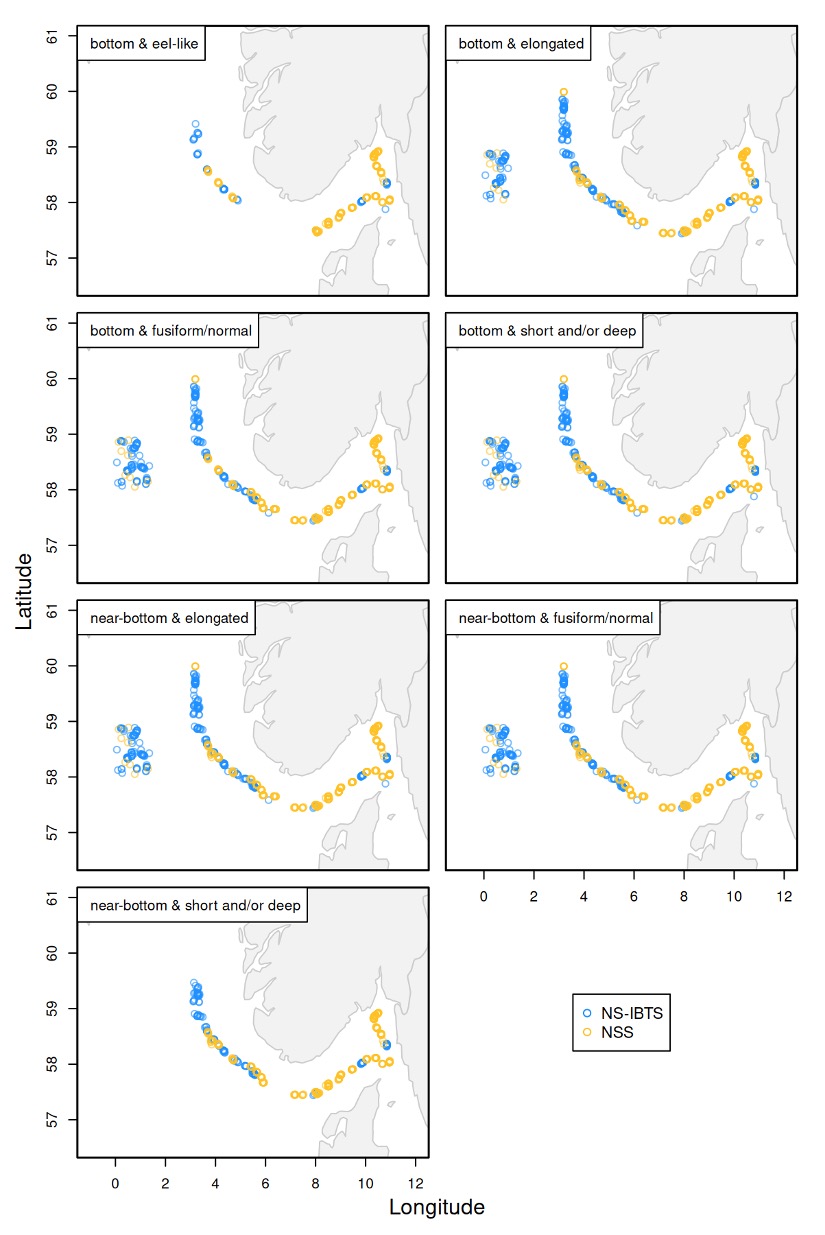
To combine the two surveys with different gears into a single model, it was necessary to account for potentially different catchability of the two surveys. As the survey catchability likely depends on the body shape of the species, species with similar morphological features were combined similarly to Walker et al. (2014). In addition, species that are associated with the seabed, such as demersal species were differentiated from species that are near or above the surface, such as benthopelagic species. The information for both categories was derived from FishBase (Froese and Pauly, 2024). Furthermore, the estimation of the gear efficiency was restricted to a time period of 2006 to 2023, and the geographical area (ICES rectangles) and depth range (120-180m) with a good overlap and sufficient observations between the two surveys (Figure S1). The spatial-temporal model for the numbers per haul was described by:

g(\mu_i)=f_1(time_i)+f_2(lon_i,lat_i)+f_3(time_i,lon_i,lat_i)+\alpha+log(\beta+5)

where:

g(\mu_i)is the link function applied to the expected value of the response variable, here the number of individuals in haul i,
f_1(time_i)is a smooth function of time,
f_2(lon_i,lat_i)is a smooth bivariate function of geographic coordinates (longitude and latitude),
f_3(time_i,lon_i,lat_i)is a tensor product smooth to capture the interaction between time and location,
\alphaIs the gear effect,
log(\beta+5)is an offset term accounting for the haul duration \left(\beta\right) of haul i plus 5 minutes according to the recommendation by Berg et al. (2024).

The estimated gear coefficients are based on groups with 3 to 20 species and are overall within a reasonable range but varied widely for 7 groups (range of 0.16-1.82, Table 1). Overall, the catchability is lower for the ST gear in comparison to the GOV gear, with the only exception of elongated species associated with the bottom having a coefficient above 1. These gear coefficients are used for the species-specific models. Supplementary Table S2 shows each species categorized by groups of habitat and body shape.

Table S3: Estimated gear coefficients between the two surveys and gears (GOV and ST) for seven groups based on habitat and body shape. N indicates the number of species included in the group.

Group	Habitat	Body shape	N	Estimate
1	bottom	eel-like	9	0.23
2	bottom	elongated	20	0.16
3	bottom	fusiform / normal	11	0.67
4	bottom	short and / or deep	8	0.45
5	near-bottom	elongated	5	1.82
6	near-bottom	fusiform / normal	6	0.22
7	near-bottom	short and / or deep	3	0.34

The temporal and spatial trends in abundance of the species were explored by means of spatio-temporal modelling, fitting Generalised additive models (GAMs) to a subset of the data representing the realised habitat for each species following the procedure described in Berg et al. (2014). The abundance was represented by the number of individuals N_i referring to the number of individuals in the i^thhaul. In the next step, the abundance and distribution were estimated for each species without estimating a gear effect but using the estimated gear coefficients as offsets (Table 1). Spatial-temporal GAMs were then used to estimate distribution maps for each species. The model describes the relationship of the numbers per haul for a specific species and external factors by:

g(\mu_i)=f_1(time_i)+f_2(lon_i,lat_i)+f_3(time_i,lon_i,lat_i)+f_4(\surd(depth_i)

+log(\alpha\beta+5).

where:

g(μ_i ) is the link function applied to the expected value of the response variable, here the number of individuals in haul i,
f_1 (time_i )is a smooth function of time,
f_2 (lon_i,lat_i )is a 2-dimensional Duchon spline on the geographic coordinates (longitude and latitude),
f_3 (time_i,lon_i,lat_i ) is a tensor product smooth to capture the interaction between time and location,
f_4(\surd(depth_i)is a smooth function of the square root of depth,
log(\alpha\beta+5).is an offset term accounting for the haul duration \left(\beta\right) of haul i plus 5 minutes according to the recommendation by Berg et al. (2024) and the estimated gear effect for that species \left(\alpha\right).

The model residuals were assumed to follow a negative binomial distribution, and a log link function was used for the dependent variable. An adequate number of knots was used for each independent term considering the dimensions of the variable. For instance, for f₁ the number of knots were set equal to the number of years of available data, and the knots for f₂ were defined based on the spatial dimensions of the area where the species was observed. If the most complex model did not converge, the model complexity was reduced in 4 steps within an iterative process, including reduction of the number of knots.

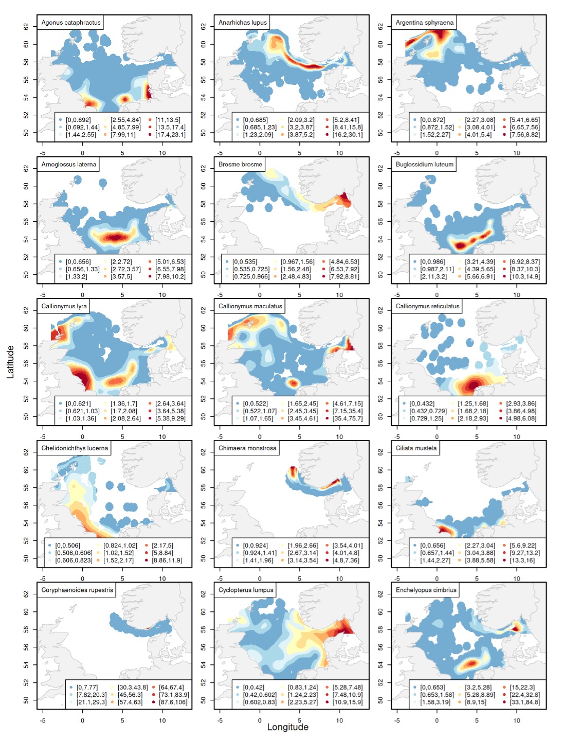
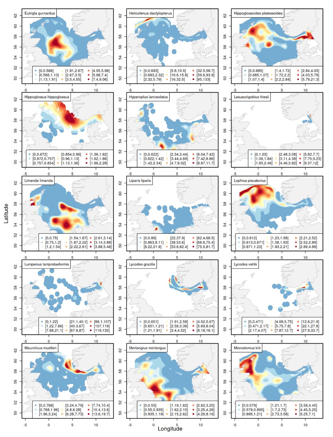
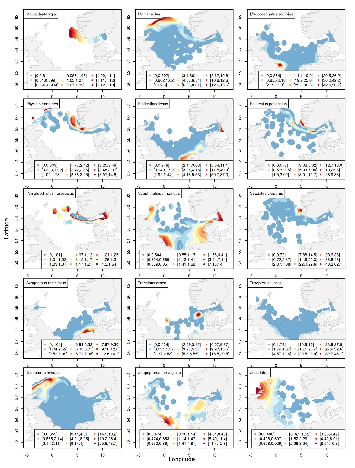
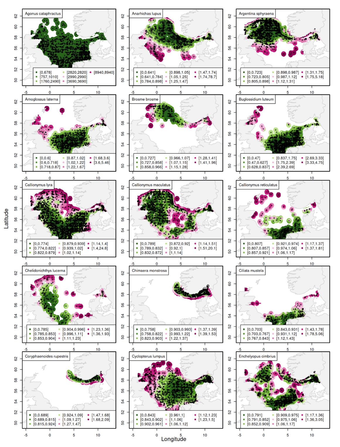
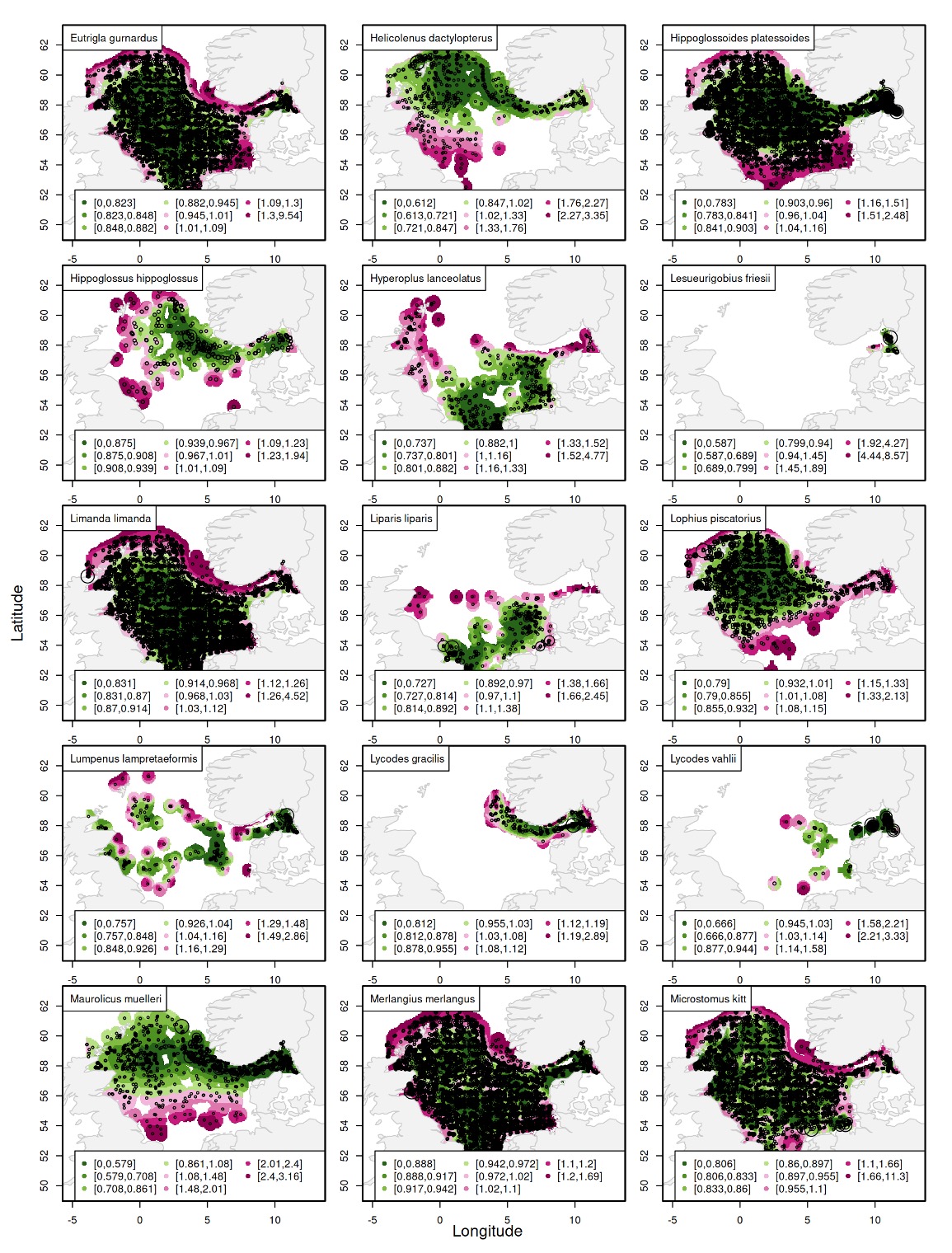
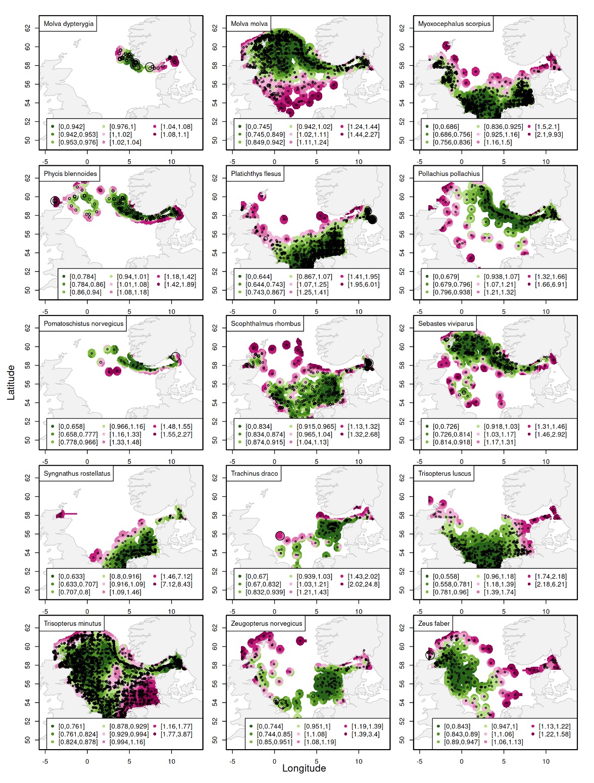
Based on the converged models for each species, the abundance was predicted for a fine spatial grid for the Skagerrak area with depth from bathymetric maps following a similar procedure as described in Berg et al. (2014): (i) dividing the realised habitat into small subareas of approximately equal size; (ii) taking the sum over all predicted abundances using the same reference gear and haul duration as well as the depth and coordinates of the grid cell. The standard deviation, coefficient of variation (CV), and 95% confidence intervals of the abundance indices were estimated based on bootstrapping. Given that n_y denotes the number of hauls each year, a bootstrap data set is created by resampling the data set with replacement, taking n_y hauls for each year from the data. All parameters (incl. smoothing parameters) and the abundance index is re-estimated for each bootstrap data set. The estimation of the standard deviation is based on 1000 bootstrap data sets. For more information about the prediction and bootstrapping procedure, please refer to Berg et al. (2014). The estimated relative abundance with 95% confidence intervals for four example species is shown in Figure 1 (please see Figure S2-4 for all 45 species).

Figure S1: Haul locations for the two surveys used to estimate the gear efficiency coefficients.

Supplementary Section 3: Spatiotemporal abundance trends for 45 species

Figure S2. Relative abundance for species 1-15 of 45 species with reliable relative abundance trend in the surveys (CV < 150%) (species with “x” in column “S” in Table S2).

Figure S3: Relative abundance for species 16-30 of 45 species with reliable relative abundance trend in the surveys (CV < 150%) (species with “x” in column “S” in Table S2).

Figure S4: Relative abundance for species 31-45 of 45 species with reliable relative abundance trend in the surveys (CV < 150%) (species with “x” in column “S” in Table S2).

Figure S5: Average distribution over period 2013-2022 for species 1-15 of 45 species with reliable relative abundance trend in the surveys (CV < 150%) (species with “x” in column “S” in Table S2).

Figure S6: Average distribution over period 2013-2022 for species 16-30 of 45 species with reliable relative abundance trend in the surveys (CV < 150%) (species with “x” in column “S” in Table S2).

Figure S7: Average distribution over period 2013-2022 for species 31-45 of 45 species with reliable relative abundance trend in the surveys (CV < 150%) (species with “x” in column “S” in Table S2).

Figure S8: Average coefficient of variation (CV) over period 2013-2022 for species 1-15 of 45 species with reliable relative abundance trend in the surveys (CV < 150%) (species with “x” in column “S” in Table S2).

Figure S9: Average coefficient of variation (CV) over period 2013-2022 for species 16-30 of 45 species with reliable relative abundance trend in the surveys (CV < 150%) (species with “x” in column “S” in Table S2).

Figure S10: Average coefficient of variation (CV) over period 2013-2022 for species 31-45 of 45 species with reliable relative abundance trend in the surveys (CV < 150%) (species with “x” in column “S” in Table S2).

Supplementary Section 4: Landings

Table S4: Species that were observed in both survey catches and commercial landings. The list of species was developed with experts from all three countries (Sweden, Norway, and Denmark).

Species	Latin	Family	Order	Danish	Swedish	Norwegian
Whiting	Merlangius merlangus	Gadidae	Gadiformes	Hvilling	Vitling	Hvitting
American Plaice	Hippoglossoides platessoides	Pleuronectidae	Pleuronectiformes	Håising	Lerskädda	Gapeflyndre
Common Dab	Limanda limanda	Pleuronectidae	Pleuronectiformes	Ising	Sandskädda	Sandflyndre
Grey Gurnard	Eutrigla gurnardus	Triglidae	Perciformes	Knurhane	Knorrhane, knot	Knurr
Rabbit fish	Chimaera monstrosa	Chimaeridae	Chimaeriformes	Havmus	Havsmus	Havmus
Lemon Sole	Microstomus kitt	Pleuronectidae	Pleuronectiformes	Rødtunge	Bergskädda, Bergtunga	Lomre
European Flounder	Platichthys flesus	Pleuronectidae	Pleuronectiformes	Skrubbe	Skrubbskädda, Flundra	Skrubbe
Roundnose Grenadier	Coryphaenoides rupestris	Macrouridae	Gadiformes	Skolæst	Skoläst	Skolest
Lumpsucker	Cyclopterus lumpus	Cyclopteridae	Perciformes	Stenbider, kulso	Sjurygg, kvabbso, stenbit	Rognkjeks
Pollack	Pollachius pollachius	Gadidae	Gadiformes	Lyssej/lubbe	Bleka, lyrtorsk	Lyr
Brill	Scophthalmus rhombus	Scophthalmidae	Pleuronectiformes	Slethvarre	Slätvar	Slettvar
Anglerfish	Lophius piscatorius	Lophiidae	Lophiiformes	Havtaske	Marulk	Breiflabb
Ling	Molva molva	Lotidae	Gadiformes	Lange	Långa	Lange
Atlantic Wolffish	Anarhichas lupus	Anarhichadidae	Perciformes	Havkat	Havskatt	Gråsteinbit
Atlantic Halibut	Hippoglossus hippoglossus	Pleuronectidae	Pleuronectiformes	Helleflynder	Hälleflundra	Kveite
Greater Forkbeard	Phycis blennoides	Phycidae	Gadiformes	Skælbrosme	Fjällbrosme	Skjellbrosme
John Dory	Zeus faber	Zeidae	Zeiformes	Sankt Petersfisk	Sanktpersfisk	Sanktpetersfisk
Tusk	Brosme brosme	Lotidae	Gadiformes	Brosme	Lubb	Brosme
Blue Ling	Molva dypterygia	Lotidae	Gadiformes	Byrkelange	Birkelånga	Blålange

Figure S11: Landings (in tonnes) by species and country for 1987 to 2023 in Skagerrak. Note that due to the scale of the y-axes some of the lower landing's years appear to be zero, however, they are only small in comparison to historical landings as Figure SX shows.

Figure S12: Landings (in tonnes) by species and country for 2013 to 2023 in Skagerrak.

Supplementary Section 5: Cephalopods

Table S5: Twenty-nine Cephalopods observed in the two surveys.

Aphia_ID	Lowest taxonomic level	Family	Order	Hauls_NOSS	Hauls_NS-IBTS	Hauls_Total
138138	Alloteuthis	Loliginidae	Myopsida	12	48	60
153131	Alloteuthis subulata	Loliginidae	Myopsida	19	3188	3207
138265	Bathypolypus	Bathypolypodidae	Octopoda	19	20	39
140596	Bathypolypus arcticus	Bathypolypodidae	Octopoda	3	0	3
11707	Cephalopoda			222	0	222
11709	Coleoidea			29	0	29
140600	Eledone cirrhosa	Eledonidae	Octopoda	0	8	8
138036	Gonatus	Gonatidae	Oegopsida	4	0	4
138278	Illex	Ommastrephidae	Oegopsida	0	212	212
140621	Illex coindetii	Ommastrephidae	Oegopsida	73	136	209
11734	Loliginidae	Loliginidae	Myopsida	0	4	4
138139	Loligo	Loliginidae	Myopsida	49	12	61
140270	Loligo forbesii	Loliginidae	Myopsida	12	1748	1760
140271	Loligo vulgaris	Loliginidae	Myopsida	7	12	19
11718	Octopoda		Octopoda	8	0	8
140605	Octopus vulgaris	Octopodidae	Octopoda	2	0	2
11760	Ommastrephidae	Ommastrephidae	Oegopsida	4	0	4
141448	Rondeletiola minor	Sepiolidae	Sepiida	1	0	1
138481	Rossia	Sepiolidae	Sepiida	0	4	4
141449	Rossia macrosoma	Sepiolidae	Sepiida	1	0	1
153083	Rossia palpebrosa	Sepiolidae	Sepiida	2	0	2
138482	Sepietta	Sepiolidae	Sepiida	14	4	18
141450	Sepietta neglecta	Sepiolidae	Sepiida	1	0	1
141452	Sepietta oweniana	Sepiolidae	Sepiida	4	156	160
11723	Sepiidae	Sepiidae	Sepiida	0	8	8
138483	Sepiola	Sepiolidae	Sepiida	8	0	8
141454	Sepiola atlantica	Sepiolidae	Sepiida	0	60	60
140624	Todarodes sagittatus	Ommastrephidae	Oegopsida	3	0	3
140625	Todaropsis eblanae	Ommastrephidae	Oegopsida	18	136	154

Figure S13: Abundance by lower taxonomic levels (first row = Family; second and third row = Genus) for NS-IBTS survey.