Hand turns down the temperature to 19 degrees Celsius on a electronic thermostat

Aerial view of skyline Helsinki. Coal for Hanasaari Power Plant
Photo: iStock

3. Impacts of the revenue cap

The aim of the revenue cap was to collect extraordinary revenues from power producers and redistribute them to consumers in order to compensate for high electricity prices. However, if the tax were to lead to reduced electricity supply, the result could be even higher prices and/or problems with security of supply. We analysed how a revenue cap on inframarginal power production technologies may affect the incentives of power producers and market outcomes and assessed the short- and long-term impacts of the revenue cap on the wholesale electricity markets. The short-term impacts are related to incentives to produce, while the long-term impacts are related to incentives to invest in new capacity.

The focus of this report is the wholesale markets for electricity, i.e., the markets for the physical electricity trade. There are three such markets with different time frames: the day-ahead market, the intraday market and the balancing market. Nord Pool is the main power exchange for electricity in the Nordic countries.

In addition to Nord Pool, physical electricity is traded bilaterally through power purchasing agreements (PPAs). There are also markets for trading financial derivatives used for hedging and/or speculation, such as the futures markets on Nasdaq OMX.

In this chapter, we start with an analysis of the impacts of the revenue cap as it was implemented in Sweden and Denmark (Sections 3.1 and 3.2). Finland implemented a temporary tax on profits for electricity producers instead of a revenue cap, which we analyse in Section 3.3. Furthermore, we discuss the impacts on competitiveness in the different countries in Section 3.4. Section 3.5 summarizes and concludes the chapter.

Main takeaways:

The revenue cap, as implemented in Sweden and Denmark, does not affect short-term incentives for inframarginal producers, i.e., producers whose marginal costs are lower than the market price.
Using a special revenue cap for producers with high marginal costs, as in Sweden and Denmark, ensures that incentives are preserved for these producers as well.
The way the tax was implemented in Sweden, with day-ahead price as the reference price and using hourly prices for settlements, does not influence producers’ short-term incentives. The impacts of using the monthly average price, as in Denmark, are not straightforward, but the incentives were preserved in Denmark as well.
Accounting for hedging agreements and PPAs ensures that the tax is based on actual realized income. This reduces the risk of potential distortions. Since a large share of production is hedged, many producers are not influenced by the tax, even when spot prices are high.
Profit taxes, as in Finland, do not influence short-run production incentives. However, the profit tax in Finland is likely to be higher than the revenue taxes in Sweden and Denmark.
Administrative costs are likely to be lower with profit tax than revenue cap. Administrative costs are likely to be lower when using the monthly average price as a tax base.
In order to maintain the incentives to invest in new capacity, the authorities should emphasize the temporary and extraordinary nature of the emergency measures.

3.1. Short-term impacts of revenue cap: Incentives to produce

The supply curve in the power market can be depicted by a merit order curve, which is a stepwise curve of different producers’ marginal costs in increasing order. Figure 3.1 shows a stylised version of the merit order curve for the Nordic power market. Marginal costs include fuel and operation and maintenance (O&M) costs of production.

For hydropower, the actual operation costs are very low, but the marginal costs include the opportunity cost (water value). The opportunity cost reflects the trade-off between producing now and postponing production until later. The opportunity cost of producing now is to lose the option to produce later.

Which technology is market-clearing (i.e., marginal) at any given time depends on several things, such as demand (which depends on day, time of day, weather, etc.), fuel and CO₂ prices, the alternative value of water in hydropower reservoirs, wind and solar conditions, maintenance schedules, and more. In addition, transmission capacity between different geographical areas may be congested, leading to different prices in different areas. In low-demand periods, wind power or nuclear power may be the marginal technologies, while in high-demand periods, gas-fired power plants are often the marginal technologies; other plants are inframarginal.

The day-ahead market uses so-called marginal pricing.

Also called pay-as-clear or uniform pricing.

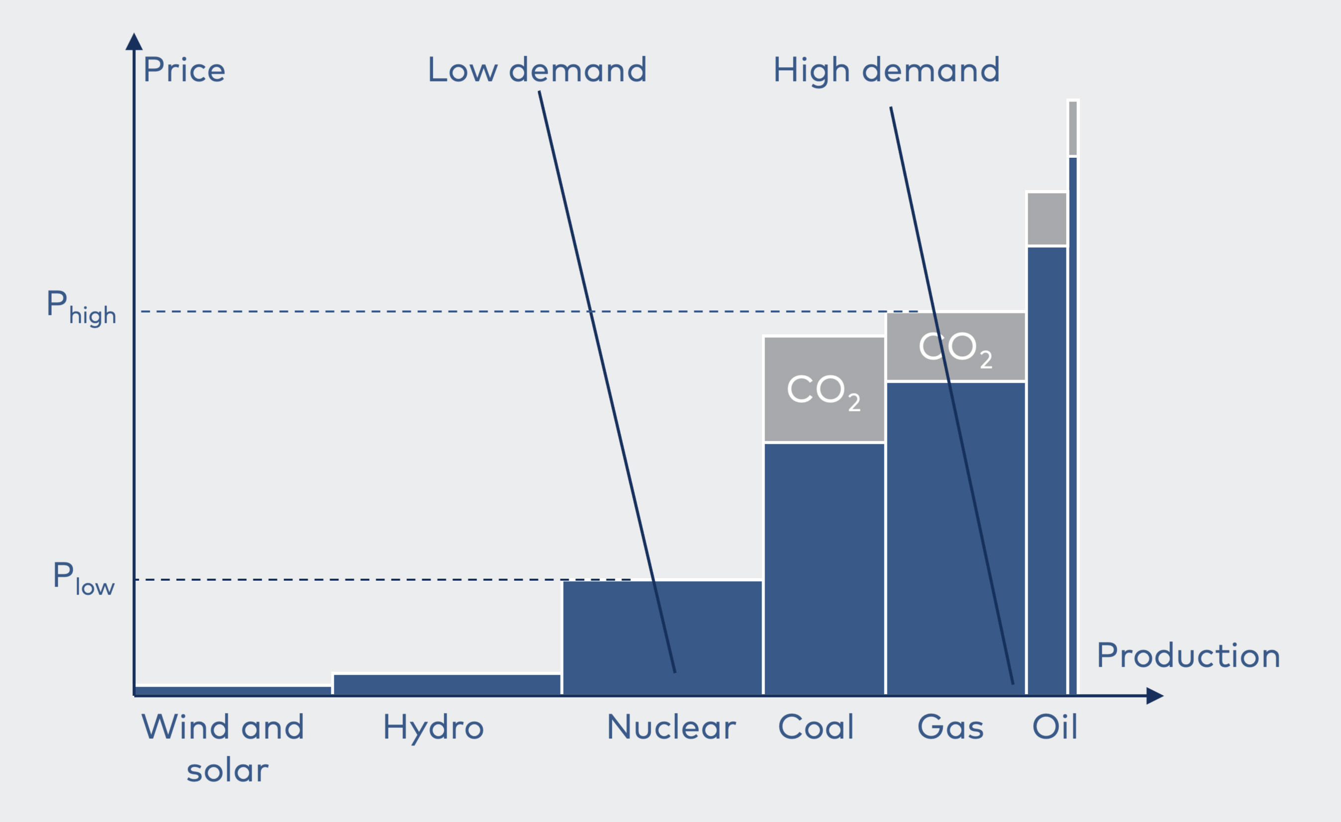
This means that all producers with accepted bids get the same price – the spot price – and all consumers pay the spot price. The spot price is the market-clearing price that ensures that demand equals supply at any given time.

Figure 3.1. Merit order curve and determination of spot price in the Nordic power market
Source: Vista Analyse

Due to uniform marginal pricing, all producers whose marginal costs are lower than the spot price (i.e., the inframarginal producers) collect rent, which is indicated as “standard rent” in Figure 3.2. This rent covers fixed costs and the return on investments for the owners. The increase in gas prices in 2022–2023 have increased the marginal costs of gas power production. This has led to higher spot prices and additional inframarginal rents for all other producers (see Figure 3.2). It is this extra rent that the authorities seek to collect from inframarginal producers. Note that the revenue cap is a tax of 90% on additional rents; the producers keep 10%.

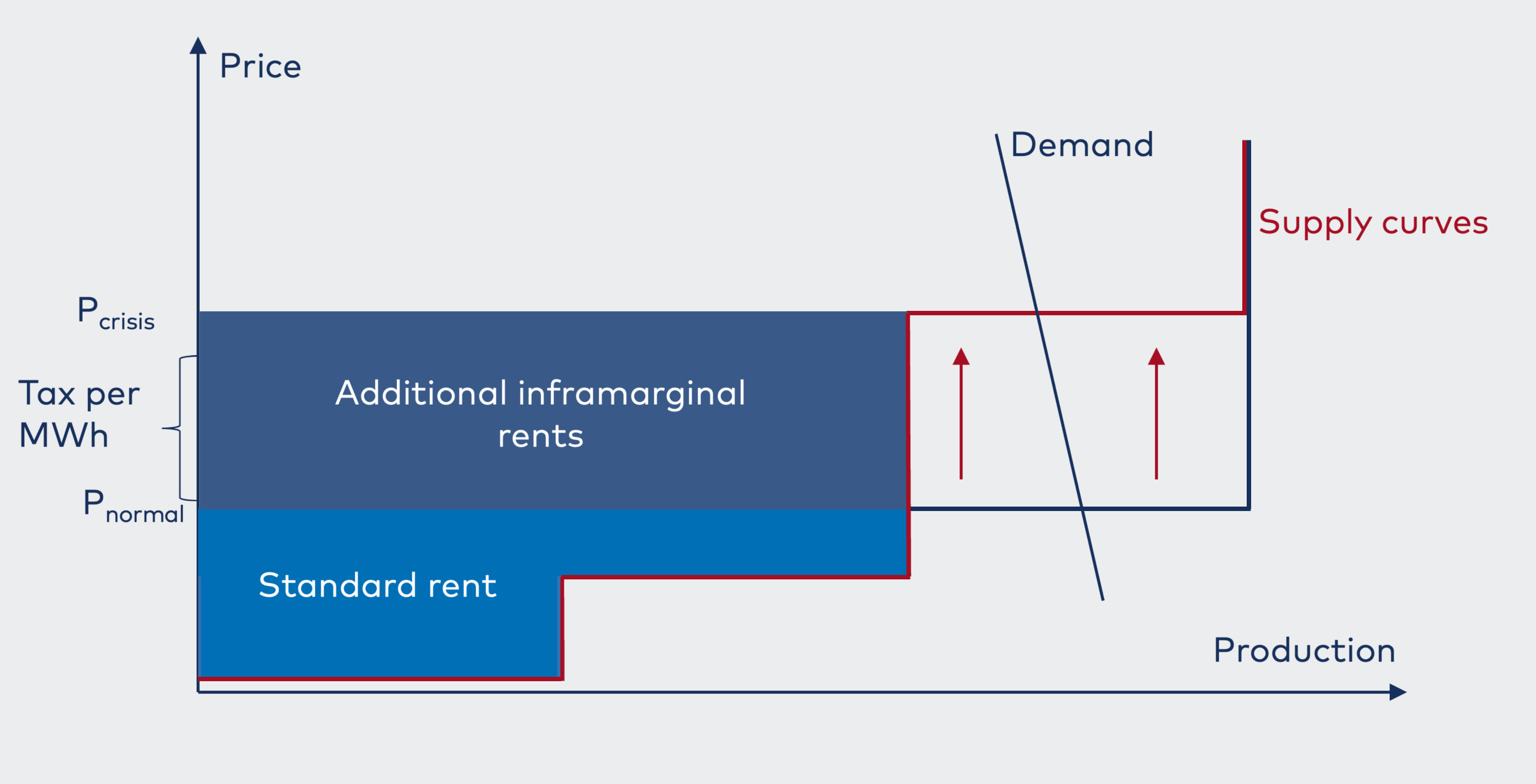
Figure 3.2. Standard rent and additional inframarginal rents due to increased power prices, and revenue tax
Source: Vista Analyse, based on Pollitt et al. (2022)

Pollitt, M., von der Fehr, N., Banet, C., Le Coq, C., Willems, B., Bennato, A.R. and Navia, D. (2022): Recommendations for a Future-Proof Electricity Market Design, Centre on Regulation in Europe (CERRE), December 2022.

In principle, a revenue cap does not affect inframarginal producers’ incentives to produce; the producers’ marginal net income from production will still be positive whenever it would have been positive without the tax. The behaviour of the producers and their bids to the market do not change. The incentive to produce is governed by a single rule: produce whenever the revenues of an additional unit (kWh) are higher than the costs of producing that unit, i.e., when marginal revenues are larger than marginal costs. Since all inframarginal producers receive the uniform price independent of their own bids, it is not rational to bid above or below the marginal costs.

Note that this mechanism is different in markets that use pay-as-bid models, such as the intra-day market.

On the contrary, by bidding anything other than marginal costs, the producer risks not activating profitable production (if the bid is too high) or operating at a loss (if the bid is too low). Thus, bid functions depend only on the producer’s own marginal costs, even with the revenue cap.

The technologies listed in the CR and those liable to the tax in Sweden and Denmark were all inframarginal technologies in periods when gas-fired power plants are price setting. Marginal producers (gas-fired power plants) were exempt from the tax. Other potentially marginal producers, such as hydropower plants with storage, were also exempt. The bid function of hydropower producers depends on expectations of future prices, and a revenue tax could affect their production incentives. There were special provisions for other high-cost producers (details in Section 3.1.1).

To conclude: in principle, a revenue cap does not change inframarginal producers’ incentives to produce. As long as the incentives to produce in the short term are preserved, the supply side will function as before. However, the devil is in the details – the specific implementation of the revenue cap may lead to changes in incentives. Therefore, we turn to an analysis of the specific details of the revenue cap in Sweden and Denmark: the special adjustments for high-cost producers, the settlement periods and the use of reference prices. The main question is whether a revenue cap, as implemented in Sweden and Denmark, influences producers’ incentives to produce and bid in the different markets.

3.1.1. Impacts of special adjustments for high-cost producers

Some of the technologies listed in the CR have high marginal costs; they are normally profitable only when prices are high. Furthermore, gas prices have not only been extremely high in the past year but fuel costs for biomass and oil have increased considerably.

Special rules were permitted for these technologies (Article 8.1b in the CR). Both Denmark and Sweden used this possibility. In Denmark, biomass- and oil-fired power plants had a special provision: the revenue cap was set as a fixed amount on top of marginal costs.

L 68 - 2022-23 (2. samling) (oversigt): Forslag til lov om et loft over indtægter fra elproduktion. / Folketinget.

In Sweden, the special cap for high-cost producers was set at 1.3 times the operation costs for producers using crude oil.

The Swedish government clarified that crude oil-fired generation plants would be taxed, but fuel oil-fired generators would not.

In both cases, these special caps ensured that marginal revenues exceeded marginal costs. Furthermore, only 90% of revenues exceeding the threshold price were taxed. These adjustments maintained the incentives to produce and contributed to the security of supply.

However, these special adjustments are an example of the regulation being administratively complicated and demanding.

3.1.2. Impacts of the settlement periods (hourly vs. monthly)

Sweden and Denmark used different settlement intervals to calculate the tax base. This had different impacts on marginal revenues and thus also on producers’ incentives. The main difference between the two settlement methods was:

The Swedish tax applied to realized revenues based on hourly prices. While the tax was calculated on a monthly basis, the revenues that formed the tax base were the sum of realized hourly earnings in so-called qualified hours (i.e., hours when the price is above the cap level), less the number of qualified hours multiplied by the cap level (see Text Frame 3.2 for the calculation). Recall that the actual revenues formed the tax base since hedging agreements and long-term contracts (PPAs) were considered. This method implies that companies were taxed for every MWh they sold at a price above the cap.
The Danish tax applied to realized revenues based on average monthly prices, which implies a monthly realized average “net price” per MWh (revenue per MWh). The tax base was calculated as 90% of total monthly revenues less 180 EUR/MWh for each MWh sold. As in Sweden, hedging agreements and long-term contracts (PPAs) are taken into account. This method implies that companies were only taxed if their realized average revenue per MWh was above the cap.

Administrative costs are likely to be lower when the monthly average price is used as the tax base, as pointed out by the Danish authorities (see Chapter 2.2.3).

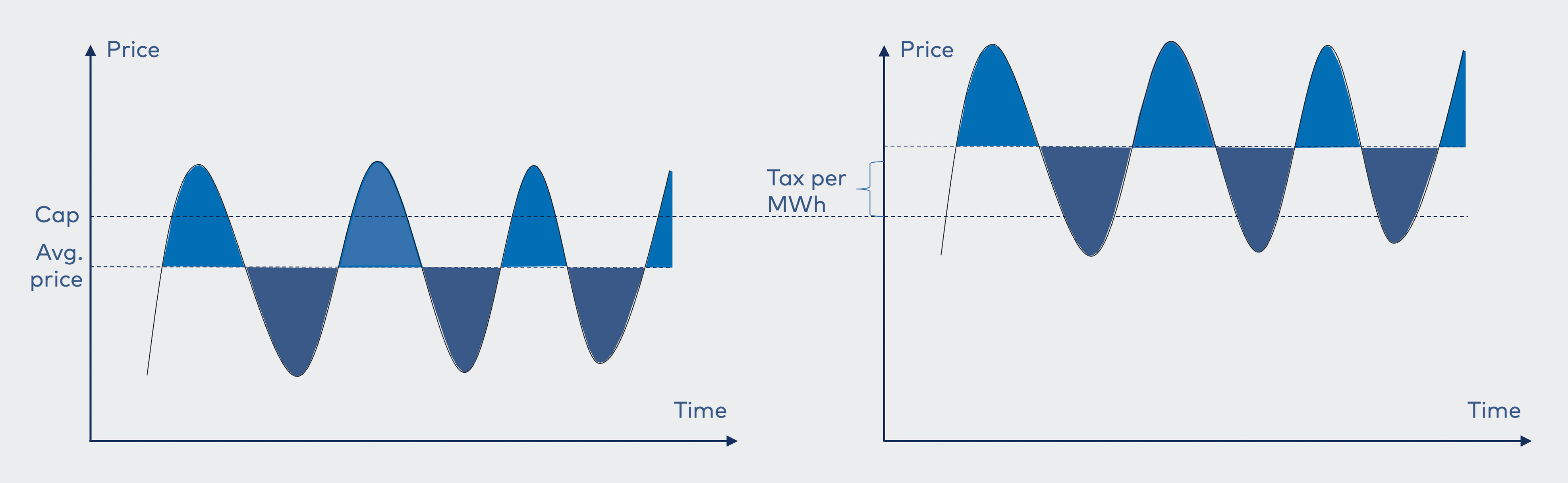
The differences between the two methods are illustrated in Figures 3.3 and 3.4. Both figures show a hypothetical hourly spot price in a month. This represents the potential marginal gross revenue per MWh for the non-hedged production of a hypothetical producer. Figure 3.3 shows that Swedish producers were taxed for all hours when the hourly price exceeded the cap level (represented by the shaded area between the price curve and the revenue cap). Danish producers, in contrast, were taxed only when the monthly average price was above the cap level, as shown in Figure 3.4. The average price is found where the light blue and dark blue areas are balanced. In Figure 3.4, the average price is below the cap; thus, the producer did not pay any tax in this case.

Figure 3.3. Swedish model: Hourly price

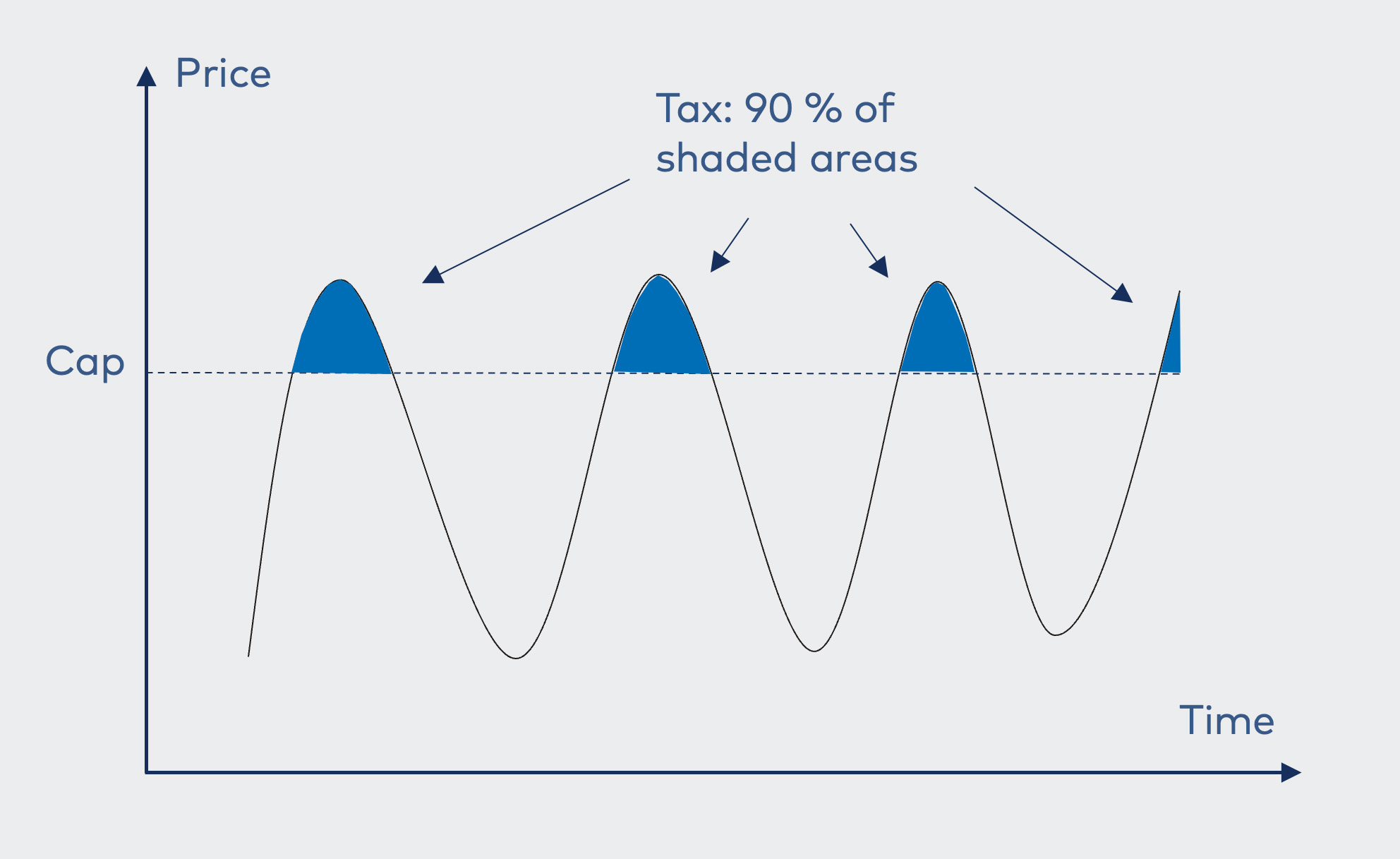
Figure 3.4. Danish model: Monthly average price

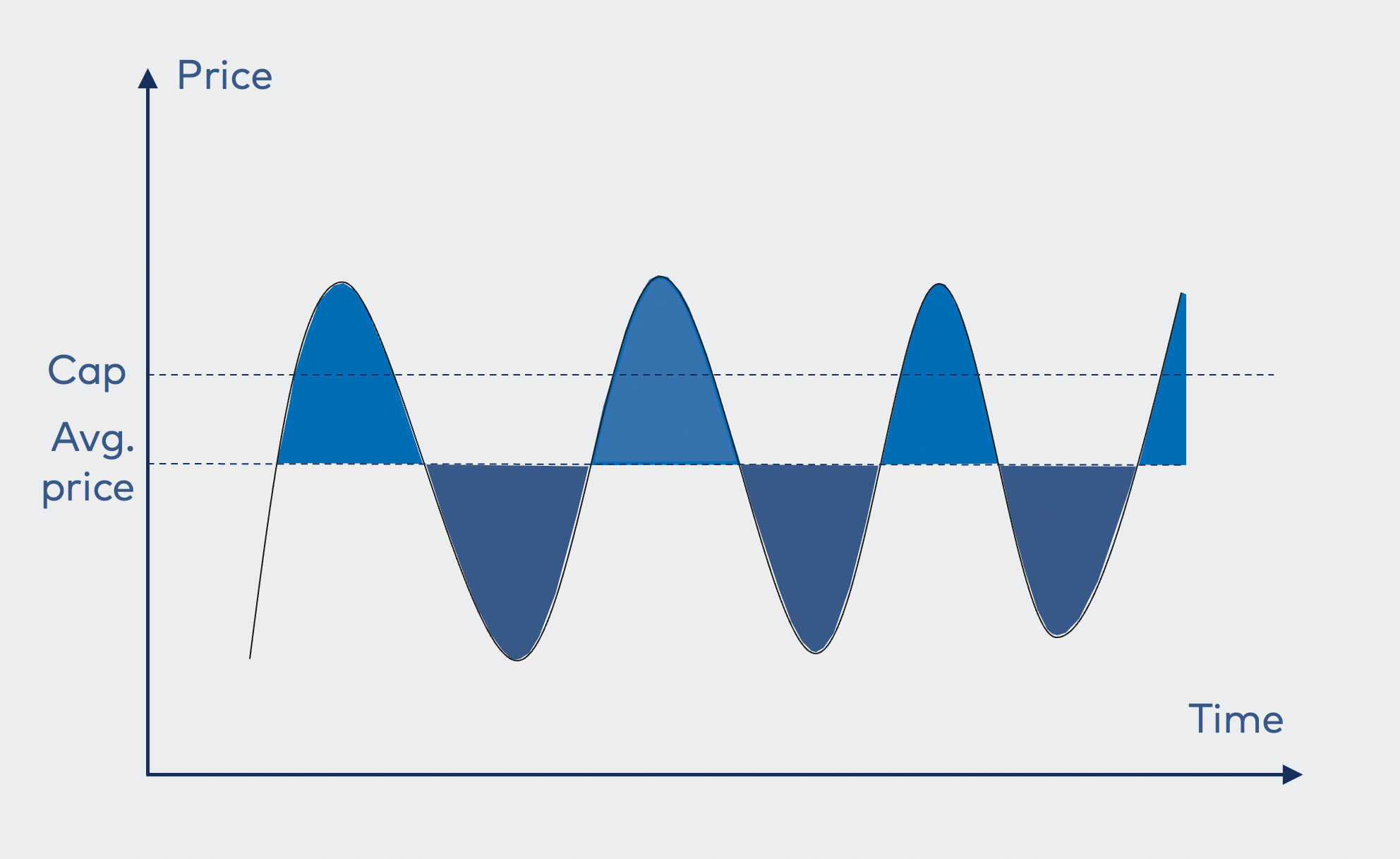
Figure 3.5. Danish model with low and high average spot prices

Source: Vista Analyse

Figure 3.5 illustrates the Danish model in more detail. The left panel shows a situation with low average prices, and the right panel shows a situation with high average prices. The revenue cap level is indicated by the dotted line crossing both panels. Producers in the left panel were not tax-liable because the average price was lower than the cap. However, the average price in the right panel is above the cap, which means that producers paid a tax of 90% for every MWh produced that month.

Note that the average prices, as shown in Figures 3.4 and 3.5, are simple averages of all hourly prices in a month, which implies that our hypothetical producer had identical production in each hour. In reality, Danish producers were taxed based on a volume-weighted average, which means that the average revenue for all producers was not necessarily equal to the simple average of hourly prices. We discuss this further below.

There are two main implications of the different schemes:

First, it is significantly less likely that the average spot price during a month is above 180 EUR/MWh than that any hours in a month will have a price exceeding 180 EUR/MWh. As shown in Figure 3.6, average spot prices in Denmark were above the cap only in December 2022 (although prices exceeded the cap in some hours every month).
The Danish government has calculated expected tax revenues using different settlement periods for December 2022–January 2023. Based on actual spot prices in the period, they showed that using monthly settlement reduced tax revenues, compared to using shorter settlement periods. Source: https://www.ft.dk/samling/20222/lovforslag/L68/spm/3/index.htm.
Prices were significantly lower in spring 2023 than in summer and early autumn of 2023 (as shown in Figure 1.1). However, it is not evident which system could provide the highest government revenues or tax burden in reality since the Swedish tax only applied until March 2023.
Second, Swedish short-term production incentives were less complicated than the incentives of Danish producers, who had to consider the effect marginal production would have on their monthly unit revenue. However, short-term production incentives were generally preserved in both countries. For a mathematical presentation of marginal net revenue calculations in the two countries, see Text Frame 3.1.

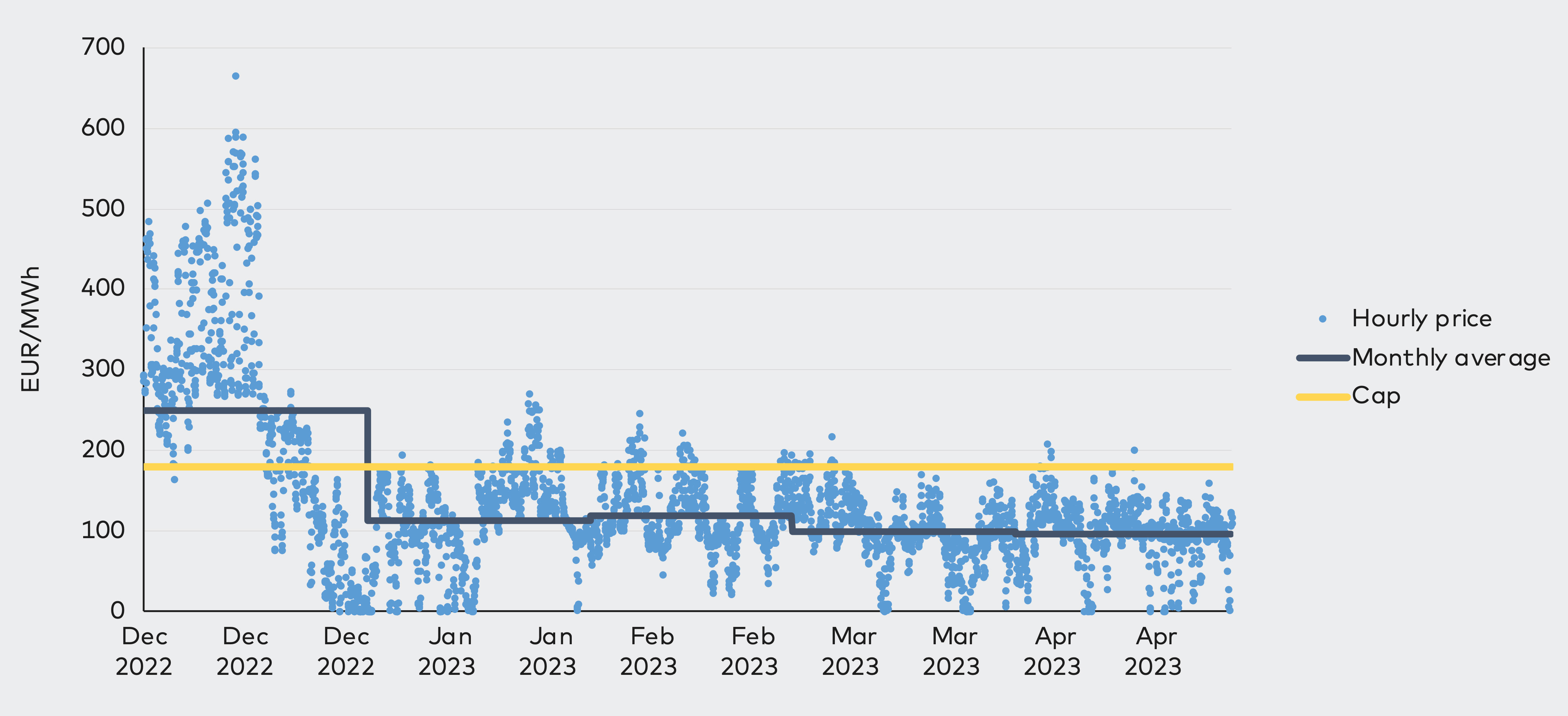
Figure 3.6. Hourly versus monthly average prices in Denmark (DK1, day-ahead)
Source: Vista Analyse, based on data from ENTSO-E

Below, we explain why short-term production incentives were preserved in general.

The short-term production incentives for Swedish inframarginal producers were unchanged because it is rational to produce, even for prices above the cap level, as long as the price covers marginal costs. Even if most of the marginal revenue above the cap level is taxed, a producer will still have a marginal income of 180 EUR/MWh plus 10% of the exceeding price. Furthermore, even if all of the revenues above 180 EUR/MWh are taxed (instead of 90%), the incentives of inframarginal producers will not be affected since marginal revenues at 180 EUR/MWh would cover marginal costs. An exception is hydropower plants with a storage capacity of less than 24 hours, which are tax liable in Sweden.

Chapter 5.4 of the Swedish bill.

A tax level of 90% (instead of 100%) would preserve correct incentives for these plants in situations where prices fluctuate at a level above 180 EUR/MWh within a day and it is possible to shift production between hours. Finally, setting the tax at 100% could have worsened incentives to produce for high-cost technologies in some situations; the special adjustments described in Chapter 3.1.1 ensure that incentives are maintained.

As mentioned, Danish short-term production incentives are not as straightforward as in Sweden, but incentives were preserved in Denmark as well. However, this is not immediately evident, though, because producers face a trade-off in some situations and spot price levels.

There are two main cases to consider. One is when the expected average unit revenue is below the cap. In this case, producers are not tax liable, and the incentives to produce are therefore identical to those in the non-tax case.

The other case is when the expected unit revenue is above the cap. In this case, producers must consider two effects of the revenue cap on their marginal revenues:

The direct effect is the marginal revenue in the hour in question, net of tax. As long as the spot price is higher than the tax payment per MWh, this effect is positive. However, in situations with high expected unit prices and low hourly prices, this effect could give producers an incentive to stop production. Consider, for example, a producer who, due to very high prices so far that month, expects to be tax liable, i.e., their unit revenue is above 180 EUR/MWh. For simplicity, we disregard any start and stop costs and other non-linearities. Then comes a period of expected low prices. Assume for simplicity that the implied average price that month is expected to be 280 EUR/MWh. This implies that producers must pay a revenue tax of 90 EUR/MWh that month on each unit sold: (280 EUR/MWh – 180 EUR/MWh) x 0.9 = 90 EUR/MWh. In hours where the spot price is below 90 EUR/MWh, for example 80 EUR/MWh, the net marginal revenue of producing electricity that hour is -10 EUR/MWh, which is negative, even if gross marginal revenue is positive. Thus, the direct tax effect in this example gives the producer an incentive to stop production altogether.
We have seen this kind of behaviour by consumers in Norway, where the household electricity price subsidy was calculated on the basis of monthly average price. Consumers were, in effect, paid to consume electricity in hours where the price was positive but where the expected subsidy made consumers’ “net price” negative. An important difference here is that the average price in Norway is not volume-weighed but completely exogenous to any single consumer. Therefore, Norwegian households faced only the direct effect and not the indirect effect.
The indirect effect on marginal revenue works through unit price. Producing in an hour with low prices will reduce the (monthly average) unit price and thus reduce the tax liability not only for current production but also for all previous production that month. Thus, the indirect effect gives producers incentives to increase production (if possible), i.e., the opposite of the direct effect in low-price situations.
Note that production incentives are preserved also in cases where the expected price is above the expected unit price. For an additional MWh supplied, tax payment increases, but gross revenue increases even more, resulting in a net positive.

Our numerical calculations indicated that the positive indirect effect is likely to be stronger than the negative direct effect in low-price situations. The reason for this is that the indirect effect affects all production hours, while the direct effect only affects a single hour.

Text Frame 3.1. Difference between Swedish and Danish short-term production incentives

In both countries, total monthly net revenues from production are given by the expression

$$ R=\underbrace{\sum_t\left(p_tx_t\right)-\sum_tC_tx_t}_{\textit{Gross revenue}}-\underbrace{0.9\left(\pi-\tau\right)\sum_tx_t}_{\textit{Tax}} $$

where

is the spot price,

is production,

is unit production cost, 0.9 captures that 90% of revenues above the cap are liable to tax,

\pi

is the settlement price,

\tau

is the cap level in EUR/MWh and subscript

indicates hour.

In Sweden,

$$ \pi=p_t $$

, since the tax was determined by the hourly spot price. In Denmark,

\pi=\overline{p}_{}

, which is the average realized price per unit sold during the month (average unit revenue). This is a volume-weighted average, so

\overline{p}=\Sigma_t\left(p_tx_t\right)/\Sigma_tx_t

, which depends on

x_t.

We suppress the time subscripts

in the following.

In Sweden, the marginal net revenue (i.e., the revenue gained or lost from producing another unit after tax) in any given hour is thus:

$$ \textit{Marginal Net Revenue}^{SE}=p-C-0.9\left(p-180\right) $$

if the price is above the cap, and

p-C

if the price is below the cap. Swedish producers thus only consider the direct effect on revenue production at any given time.

In Denmark, the marginal net revenue is more complicated because producers also had to consider how production

\left(x\right)

at any time would affect the average unit revenue

\left(\overline{p}_{}\right)

$$ \textit{Marginal Net Revenue}^{DK}=\underbrace{p-C-0.9\left(\overline{p}-180\right)}_{\textit{Direct}}-\underbrace{0.9\frac{\mathrm{d}\overline{p}}{\mathrm{d}x}\sum x,}_{\textit{Indirect}} $$

where

d\overline{p}/dx<0

for spot prices below the expected monthly unit revenue. The direct effect is the marginal revenue for the specific hour, net of tax. This expression looks similar to the Swedish model but note that the tax term includes average unit revenue and not hourly price. The indirect effect is the impact on marginal net revenues resulting from the marginal change in unit revenue from current production applied to all monthly production.

3.1.3. Impacts of using the day-ahead price as a reference price on incentives to shift supply between markets

In Sweden, the day-ahead price was used as a reference when calculating revenue from all markets (adjusted for hedging agreements). For example, if the day-ahead price was 190 EUR/MWh for a given hour and a producer received 210 EUR/MWh from supplying to the intraday market for the same hour, this producer was taxed according to 190 EUR/MWh, even if the realized revenue per MWh on the intraday market was higher. The same applied if the price on the intraday market was lower – producers were taxed according to the day-ahead price.

In Denmark, however, the actual price on the relevant market was used as the tax base (adjusted for hedging agreements). This was directly stated in the provisions and was an implication of the monthly settlement interval chosen in Denmark. Since the average revenue per MWh during a month was the tax base, revenue from markets with relatively higher prices increased producers’ average revenues and thus the tax base.

Some Swedish public consultation statements argued that using the day-ahead price as a reference could have reduced liquidity in day-ahead markets and increased liquidity in markets closer to real time because expected prices are often higher in these markets.

See, for example, the consultations statement from Nord Pool.

Since the day-ahead price was used as a reference, suppliers could withdraw supply from the day-ahead market, hoping to increase actual revenues while the tax base stayed the same. Prices on the day-ahead market could increase due to reduced supply or increased opportunity cost of supplying on the day-ahead market because of higher expected returns on the intraday and balancing markets.

However, producers’ incentives will not differ from those before the tax, regardless of whether a reference price is used. A producer has an incentive to produce in Market B if the expected marginal net revenue in Market B is higher than in Market D

\left(MR_B>MR_D\right)

If the price from Market D is used as a reference, the producers have incentives to shift production to Market B if

\begin{align} & p_B-0.9\left(p_D-180\right)>p_D-0.9\left(p_D-180\right) & \\ & p_B>p_D & \end{align}

Because the tax term cancels out, it is clear that producers shift production only if the gross price is higher in Market B.

If actual prices are used to calculate the tax in both markets, the decision rule is:

\begin{align} & p_B-0.9\left(p_B-180\right)>p_D-0.9\left(p_D-180\right) & \\ & p_B-0.9p_B>p_D-0.9p_D & \\ & 0.1p_B>0.1p_D & \\ & p_B>p_D & \end{align}

By comparing the two scenarios, one can see that the incentives depend only on (gross) price. Producers shift supply between markets only if the price in one market is higher than in the other.

These results apply even if only one market price is above 180 EUR/MWh while the other is below. If a reference price is used, the tax term on each side of the inequality either cancels out (if the reference price is above the cap) or does not enter at all (if the reference price is below the cap). In both cases, the gross spot price determines production incentives.

If, on the other hand, actual market prices are used, we have (for

p_B>180

and

p_D<180

\begin{align} & p_B-0.9\left(p_B-180\right)>p_D & \\ & 0.1p_B+162>p_D & \end{align}

This inequality holds for all situations where

$$ p_B>180 $$

and

p_D<180

, which means that incentives are maintained even in situations where one market is taxed and the other is not.

The opposite case, with

p_B<180

and

p_D>180

, gives the equivalent inequality as the first case, only with subscripts switched around (remember that the no-tax incentive is still to supply to the market with the highest price). Therefore, the result holds the other way as well.

Hence, using the day-ahead price as a reference price for all markets does not affect incentives to shift supply between wholesale markets (from day-ahead to intraday).

However, government tax revenues are affected by the choice of reference price. If the day-ahead market on average has the lowest prices of the three wholesale markets, using the day-ahead price as a reference price will, all else being equal, give a lower government tax income than using actual prices.

3.1.4. Impacts of incentives on the intraday market

In contrast to the day-ahead market, which uses marginal pricing, the intraday market uses a pay-as-bid model (see Text Frame 3.2). In the intraday market, suppliers face a trade-off when submitting their bids because they are paid their bids and not the market-clearing price. On the one hand, sellers are tempted to bid above their marginal costs since they are paid their bids. On the other hand, bidding too high involves the risk of not being dispatched and gaining nothing.

With complete information, pay-as-bid markets are equivalent to pay-as-clear markets. However, in reality, information is incomplete, which may distort the merit order as a result of information asymmetry.

The marginal revenues of producers thus depend on their bids and their marginal costs, and their bids depend on expected average prices (and marginal costs).

As implemented in Sweden, a revenue cap uses the day-ahead market price as the reference price. Thus, the revenue cap will not affect behaviour in the intraday market because the optimal bid functions are not affected by the day-ahead price, or the day-ahead price affects the expected prices on the intraday market in the same way for all agents, and this price is common knowledge to all bidders.

The Danish implementation did not have an hourly settlement but used total revenues to calculate the tax base. Thus, it was still optimal to maximize revenues for given marginal costs, which implies that behaviour was unaffected by the tax.

Hence, the implementations in Denmark and Sweden ensured that incentives in the intraday market were not affected.

Text Frame 3.2. What is the intraday market?

The intraday market is a market of physical power delivery where participants adjust their positions between the closing of the day-ahead market and the time of delivery. In the Nordic countries, the intraday market is called Elbas (Electricity Balance Adjustment System) and is operated by Nord Pool. Elbas is used for trading internally in a country and across borders.

The intraday market continually connects buyers and sellers who make bilateral trades. Market participants place buy and sell orders for energy and price combinations for certain time periods (e.g., sell 50 MWh for 47 EUR/MWh at 12:00–13:00 CET).

The intraday market settles orders using a pay-as-bid model: sellers are paid their asking price, and buyers are paid their bidding price. Nord Pool matches orders that intersect (i.e., where the price limit of the sell order is not higher than the price limit of the buy order), and the settlement price for each trade is determined by the order first placed (i.e., the asking price if the sell bid came first, and the bid price if the buy bid came first). Intraday auctions (or “batch matching”) are used in certain cases.

See https://www.nordpoolgroup.com/48fa80/globalassets/download-center/cacm-regulation/public-description-of-the-continuous-trading-matching-algorithm.pdf

3.2. Long-term impacts of revenue cap: Incentives to invest

Main takeaways:

Investment decisions depend on expectations about future prices and future cash flows.
A revenue cap may influence expectations about future taxes, which may reduce the net present value of investments.
Setting the revenue cap level above expected peak prices contributes to preserving incentives to invest.
It is vital that authorities emphasize the temporary and one-time nature of such taxes in order to maintain investment incentives.

Many inframarginal technologies have low operation costs but high capital costs. Capital costs are recouped through profits earned in periods when the spot price is higher than the marginal cost. This is shown as standard and additional inframarginal rents in Figure 3.2. A revenue cap reduces the revenue of inframarginal producers by capturing part of the additional inframarginal rents. This reduces the after-tax profitability of investments and might make some projects unprofitable.

Investors find it profitable to invest if the net present value of a project is positive. Future cash flows are uncertain, however, and investors form expectations about future cash flows based on their beliefs about the future. Therefore, the main question is whether features of the current crisis and governments’ responses thereto may significantly alter expectations about the future.

In general, uncertainty about the future is a cost that investors include in their calculations, effectively raising the required yield. Sudden, unexpected taxes may increase the general uncertainty about future income and cost streams. This raises the discount rate used in net present value calculation, as investors prefer a more certain income in the near future over a more uncertain income in the distant future. Hence, a revenue cap may lead to a higher discount rate and fewer investments. This uncertainty is not unique to the electricity industry but applies to all industries in the economy. There is always a risk that new policies and taxes will be implemented, for example, after an election.

A related question is at which level the cap is set, i.e., which price level is perceived as “extraordinary”. The revenue cap implemented in Sweden and Denmark was set at levels exceeding expected peak prices before Russia’s invasion of Ukraine, according to the CR and an impact analysis by the Swedish government.

The CR, recital 28.

Tillfällig skatt på vissa elproducenters överintäkter Fi2022/03328 (12 December 2022).

This implies that the actual marginal revenues after tax are higher now than what was expected before the war and sufficient to generate profitability for investments. Thus, one may induce revenues to cover capital costs, and only windfall profits are collected by emergency measures, not ordinary return on investments.

Electricity prices have been much higher in 2022–2023 than in previous years and will be higher than expected in the future. It is unlikely that any investor would invest solely on the basis of the present extraordinary high prices, as investors consider long-term expectations about prices. The present uncertainty about prices and taxes may cause some investors to postpone making decisions.

To conclude, the main question is whether investors believe that policymakers will implement revenue caps or other extraordinary measures again whenever prices are extraordinarily high, or whether they perceive these measures as temporary, one-time measures due to an extraordinary situation. The CR was introduced as an exceptional, targeted and time-limited measure. The authorities can avoid negative impacts on investments by emphasizing that these measures are extraordinary indeed, that they were introduced as a response to a crisis, and that they are unlikely to be used again.

3.3. Impacts of the temporary tax on profits in Finland

Main takeaways:

Profit taxes do not affect short-run production incentives.

The profit taxes in Finland apply to all power production technologies. Hence, administrative costs are lower than in Sweden and Denmark.
The Finnish tax is ex post higher than the revenue tax in Sweden and Denmark; average spot prices have been below the equivalence level of 280 EUR/MWh.
The profit tax does not influence the relative profitability of different investments in electricity industry but may influence the allocation of capital between different sectors of the economy.
The authorities should emphasize the temporary and extraordinary nature of the tax to reduce negative effects on investments.

Finland implemented a tax on profits instead of a tax on revenues. In Finland, 30% of power producers’ profits exceeding an annualized return of 10% on equity are taxed. The profit tax was calculated to be equivalent to a revenue cap for average spot prices of 280 EUR/MWh from December 2022–June 2023.

The law does not discriminate between generation technologies but applies to all technologies. The tax is to be levied on profits during the 2022 and 2023 tax years, in addition to the ordinary corporate income tax.

For further details, see Chapter 5.1.2 of the Finnish bill.

A profit tax is easier to implement than a revenue cap. Therefore, administrative costs are lower.

3.3.1. The Finnish profit tax will not affect wholesale markets in the short run

Profit taxes do not affect short-run behaviour. Profit-maximizing firms have incentives to maximize profits even if a share of profits is taxed. Behaving otherwise, for example, by shifting production schedules or shutting down, would reduce profits if pre-tax activities were optimal. Thus, rational agents in the electricity sector behave as before and offer the same supply in the same markets as before. Hence, wholesale markets are likely to be unaffected by a temporary profit tax in the short run.

3.3.2. Will the Finnish profit tax affect investments in the long run?

The tax on profits has reduced the expected after-tax net present value of investment projects in the electricity sector. This alone does not affect the relative profitability between different projects or different electricity generation technologies, but it may affect the allocation of (scarce) capital between different sectors of the economy and foreign investments.

The effect on investments depends on expectations, as discussed in Section 3.2. If the tax is believed to be a temporary measure due to an extraordinary crisis, investments are not affected. However, if the crisis has altered investors’ expectations about future prices, profits and government reactions, investments may be affected.

Expectations of similar taxes in the future are tied to agents’ expectations about future prices: if investors believe that no extraordinary taxes are introduced when prices and profits are “ordinary”, incentives to invest will not change. If some, but not all, of the excess profits in “extraordinary” periods are expected to be taxed, investments may decrease compared to the same situation without taxes because investors may use scarce capital in other sectors.

3.4. Impacts on competitiveness between countries

It is relevant to consider whether the differences in the implementation of the tax impacts the competitiveness of the Nordic countries.

In contrast to electricity producers in Sweden and Denmark, where the tax was implemented as a revenue cap, electricity producers in Finland are taxed at 30% of profits that exceed a 10% return on equity. The profit tax in Finland was calculated to be equivalent to a revenue cap for average spot prices of 280 EUR/MWh in the period December 2022–June 2023. All else being equal, when actual average spot prices are lower than 280 EUR/MWh, the tax burden on companies (and government proceeds) would be higher in Finland than in Denmark and Sweden, given that Finnish producers earn profits that are above 10% return on equity. However, average spot prices have been significantly lower than 280 EUR/MWh since January 2023 (see Figure 1.1). Thus, on average, Finnish producers are likely to be taxed at a higher rate than producers in Sweden and Denmark.

Figure 3.7 illustrates the differences between the two tax systems. The figure shows how profit per unit after tax varies with spot prices, given that the producer is expected to exceed a 10% return on equity. We also assume that marginal costs are covered (which they must be for production to be profitable) and constant (which is a minor simplification).

The kinked line illustrates profits under the revenue cap system. For prices below the cap (180 EUR/MWh), marginal profits increase in a one-to-one relationship with the spot price. For prices above the cap level, the profit line is less steep since a share of the revenues is taxed.
The straight line illustrates profits under the profit tax system. The relationship between price and profits is less than one-to-one because a share of profits is taxed.
The two systems yield the same result when the average spot price is 280 EUR/MWh. For average prices below this, profits after tax are lower in the profit tax system than in the revenue cap system. The opposite is true for an average price higher than 280 EUR/MWh.

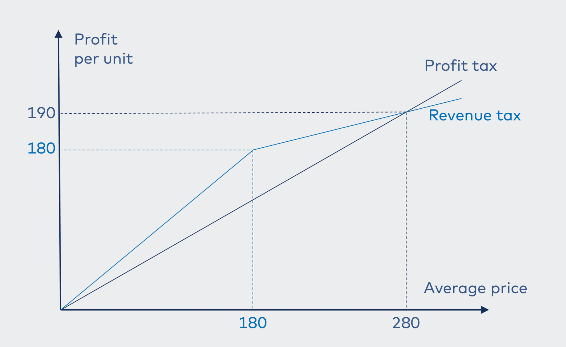
Figure 3.7. Profits per unit and prices under different tax systems
Source: Vista Analyse

It is important to note that profit per unit strictly increases with electricity prices in both systems. This means that the short-term incentives to produce are maintained for both systems. Producers cannot choose where to supply their power; incentives are therefore maintained even with cross-border power trade since producers get the price in their own bidding zone.

The potential long-term impacts of different tax systems relate to investments. Both the revenue cap and the profit tax are temporary and extraordinary measures, and it is not clear to what extent these measures may influence investments. In general, having different tax systems in the Nordic countries may introduce wedges between expected after-tax profitability, which could affect how competitive the countries are in attracting investment capital. Hence, similar tax systems would avoid changes in competitiveness.

3.5. Concluding remarks about the revenue cap and the profit tax

We assessed the short- and long-term impacts of the revenue cap on wholesale electricity markets. The main question was whether the revenue cap on inframarginal technologies will affect the incentives of power market participants. The short-term impacts are related to incentives to produce, while the long-term impacts are related to incentives to invest in new capacity.

3.5.1. Short-term impacts

Our main findings related to the revenue cap in Sweden and Denmark include the following:

In principle, the inframarginal producers’ incentives to produce are not affected by a revenue cap: producers will produce as long as their marginal revenues are higher than their marginal costs.
The way the tax was implemented in Sweden, with the day-ahead price as the reference price and hourly prices for settlements, does not influence producers’ short-term incentives. The short-term incentives for Danish producers are more complicated, but incentives are preserved here as well.
The actual prices obtained by the producer form the tax base. Hence, if a producer has hedging agreements or power purchasing agreements (PPAs) and does not earn a market price exceeding 180 EUR/MWh, the tax does not apply. The share of hedging agreements in the Nordic market is relatively high, especially for wind and solar power producers, which are hedged to a large degree; therefore, a large share of production is not influenced by the tax.
Administrative costs are likely to be lower with the monthly average price as the tax base.
Special provisions for high-cost producers (biomass- and oil-fired power plants) ensure that their incentives are preserved as well, thus ensuring security of supply.

Our main findings about the profit tax in Finland are as follows:

A profit tax does not distort short-term production incentives. Profit-maximizing firms will still have incentives to maximize profits even if a share of profits is taxed. Thus, rational agents in the electricity industry behave as before and offer the same supply in the same markets as before.
A profit tax is easier to implement and has lower administrative costs than a revenue cap.
The present profit tax implies a higher tax level in Finland than the revenue tax in Denmark and Sweden. While this does not influence short-term incentives, it influences competitiveness and may influence long-term investment decisions.

3.5.2. Long-term impacts

The potential long-term impacts relate to incentives to invest. Investment decisions depend on expectations about future prices and cash flows. Therefore, the main question is how these crisis measures may influence expectations about the future – whether investors believe that policymakers will implement a revenue cap or a profit tax (or other extraordinary measures) whenever prices are extraordinarily high. If they believe that a similar tax will be introduced in the future, the expected after-tax profitability of new investment projects will be reduced, and investments may be reduced as well. In order to maintain incentives to invest, it is important to emphasize that the measures were introduced as a response to an extraordinary crisis and not as regular taxes.

Electricity prices are much higher now than they were before 2021. One may note that investments have been planned and carried out at much lower prices than those of today. However, uncertainty about market conditions in general – prices and taxes – may cause investors to postpone making decisions.

It is also worth noting that the differences in the implementation of the measures may lead to changes in competitiveness between countries. This could have long-term impacts, such as investments being “moved” from one country to another. The negative effects on investment can be mitigated by communicating that these crisis measures are unlikely to be used again.

Hence, we conclude that if investors believe that the current crisis measures are indeed exceptional, targeted and time-limited, as is stated in the Council Regulation, the long-term incentives to invest should not be affected. It is crucial that the authorities emphasize the temporary, one-time nature of the extraordinary measures.