Nordic Economic Policy Review 2023

Frederik Silbye and Peter Birch Sørensen

We analyse the extent to which the climate effect of unilateral climate policy in Nordic frontrunner countries may be nullified by the mechanics of the European Emission Trading System (ETS) in light of the recent tightening of the system. We find that national initiatives to reduce emissions from the domestic ETS sector are likely to reduce total EU-wide emissions due to the endogeneity of the cap on ETS emission allowances. We also examine the cost-effective design of the unilateral climate policy of an EU frontrunner country, given the design of EU climate policy. Finally, we show that if the policy goal is to maximise national welfare, a uniform domestic carbon price across sectors is only optimal under special circumstances, and we highlight the importance of trade in emission rights and carbon leakage for optimal policy design.

Keywords: EU climate policy, Optimal unilateral climate policy, European Emissions Trading System

JELcodes: Q48, Q52, Q58.

Despite the recent increase in the level of ambition of EU climate policy reflected in the commitment to reduce EU greenhouse gas emissions by 55% by 2030 relative to 1990, the Nordic members of the EU have adopted national targets for emission cuts that go even further. For example, the Danish Climate Act of 2020 obliges the government and Parliament to secure a 70% cut in total domestic emissions by 2030 and to aim at national climate neutrality no later than 2050. Finland aims at a 60% reduction of domestic emissions by 2030 and strives to achieve climate neutrality by 2035, in part through carbon sequestration in the large Finnish forests, and Sweden targets a 63% cut in emissions by 2030 and net zero emissions no later than 2045.

Small countries like those in the Nordic Region only account for a tiny fraction of global greenhouse gas emissions, so why should these countries set targets for emission cuts that go beyond their obligations towards the EU, despite their negligible direct impact on the global climate? This question has previously been thoroughly discussed in an article by Greaker et al. (2019) in this journal. One normative argument for an ambitious unilateral climate policy is inspired by the philosopher Immanuel Kant (1785/1993), who argued that moral actors should act in the same way as they would like others to act. Since it is generally agreed that worldwide, countries are not doing enough to stop global warming, and since all countries would presumably like to avoid catastrophic climate change, a Kantian approach would morally oblige each individual country to increase its effort at greenhouse gas abatement, even if others do not immediately follow suit.

A more common justification for an ambitious unilateral climate policy is that a frontrunner country may inspire other countries to pursue more ambitious policies by demonstrating that abatement costs are lower than previously expected or by developing new green technologies that help other countries reduce their abatement costs. To the extent that reciprocity mechanisms are at work in international negotiations on climate policy, frontrunner countries may also be able to exert stronger pressure for a tightening of emission reduction targets in other countries.

Unfortunately, there is also a possibility that some countries will find it less urgent to cut their emissions if other countries are doing the job for them by adopting more ambitious targets for emission cuts. However, such a free-rider approach seems unlikely to emerge if the frontrunner countries are small and only have a tiny direct impact on the global climate.

In this paper, we take as a given that the Nordic EU member states wish to move faster towards climate neutrality than the rest of the EU. We then discuss two major issues. First, to what extent will the direct climate effect of unilateral climate policy in a small Nordic country be nullified by the mechanics of the European Emission Trading System (ETS), given the new and tighter rules for the system recently agreed within the EU? Second, what is the cost-effective design of the unilateral climate policy of an EU frontrunner country, given the design of EU climate policy?

The first of these issues is analysed in Section 2 of the paper, and the second issue is addressed in Section 3. Section 4 contains our concluding remarks.

Nowhere is the potential conflict between European and national climate policy as evident as in the sector covered by the European Emissions Trading System (ETS), i.e. heavy industry, power plants and intra-EU aviation, which accounts for around 40% of total EU emissions. Here, the EU controls emissions by issuing new allowances. The ETS is a cap-and-trade-system, and in the textbook version of such a system, the cap is exogenous and fixed (Stavins, 2019). In the EU, a fixed total cap on ETS allowances would mean that any action taken by an individual member state to reduce emissions from the domestic ETS sector would release a corresponding amount of ETS allowances for use in other EU countries. Hence domestic emissions would simply 'leak' to other parts of the EU, and the leakage rate – defined as the increase in foreign emissions divided by the cut in domestic emissions – would be 100%, as the total EU emissions would remain the same.

In the following, we will question the premise of a fixed cap on total ETS emissions. Two arguments support the notion that the cap, to some extent, is endogenous and that it can be affected by the actions of individual member states. First, we explore the role of the Market Stability Reserve in the ETS, which has the power to cancel allowances. Second, we discuss the cap as the result of political negotiations and how the outcome of these negotiations can be influenced by national climate policies.

As noted, the textbook version of a cap-and-trade system has a fixed cap. However, ETS has moved beyond the simple world of the textbook by introducing the Market Stability Reserve (MSR). The reserve absorbs emission allowances when the allowance surplus in the market is large, and it releases allowances back to the market when the surplus is small. The critical element here is that the size of the MSR is limited. If the number of allowances in the MSR exceeds an upper limit, the exceeding allowances are permanently cancelled. Hence, it is no longer certain that the issue of an additional allowance will lead to the emission of an additional ton of CO₂e at some future point in time. The consequence is that the ETS cap has become endogenous, and individual countries may attempt to reduce overall emissions in the system by adding to the allowance surplus. For instance, a national policy initiative that reduces emissions will release allowances that add to the surplus, and some of these allowances will enter the MSR. If the upper limit on the MSR is binding, the allowances are permanently cancelled. The bottom line is that individual nations may affect EU-level emissions, and this reduces carbon leakage below 100%. This effect is thoroughly described in the literature (Perino, 2018, Silbye & Sørensen, 2019, Beck & Kruse-Andersen, 2020).

Will the ETS reform agreed in December 2022 change the mechanics of the system? Following this reform, fewer new allowances will be issued, and this may lead to a lower market surplus and, hence, less endogeneity of supply. Two questions are relevant for policy makers: (i) What is the magnitude of the endogeneity through the MSR, and (ii) in which time period is the endogeneity active? Before addressing these two questions, gaining a better understanding of the mechanisms of the MSR will be instructive.

When the total allowance surplus in the ETS exceeds 833 million tonnes of CO₂, 24% of the surplus is placed in the reserve. However, if the surplus is between 833 and 1096 million, the intake is the difference between the surplus and the 833 million, and this effectively raises the marginal intake rate to 100%. This is an important new amendment to the intake rule, introduced to avoid threshold effects. The surplus is calculated by the end of each calendar year, and allowances are then placed in the MSR over a period of 12 months starting from 1 September the following year. When the surplus falls below 400 million, an amount of 100 million allowances is released to the market. Figure 1 illustrates the net intake rule.

Figure 1. Net intake rule of the Market Stability Reserve

The recent ETS reform will also affect the maximum size of the MSR stock. Before the reform, the stock could not exceed the total volume of allowances auctioned during the previous year. However, the reform changes the upper bound of the MSR stock to a fixed limit of 400 million. As previously mentioned, allowances in excess of the MSR cap are cancelled.

To answer the two questions (i) and (ii) above, it is crucial to know if and when the allowance surplus is larger than 833 million and if and when the MSR stock hits its ceiling. In order for a national climate effort to have a long-term ETS leakage rate significantly below 100%, there must be several years where the surplus is large such that there is time for the released allowances to be soaked up by the MSR or at least one year with a surplus between 833 and 1096 million yielding a 100% intake rate. In these years, the MSR limit must also be binding, such that the marginal allowance in the reserve is cancelled.

We have used the forecasting model presented in this journal by Silbye and Sørensen (2019) to predict the evolution of the ETS implied by the reform of the system agreed in December 2022. The details of the model are documented in the Appendix to Silbye and Sørensen (2019, pp. 98–101). The model assumes that companies covered by the ETS minimise their total costs, including the costs of ETS allowances. In any given year, this leads to a downward-sloping demand curve for allowances. Over time, the demand curve shifts down due to increases in energy efficiency, the development of new green technologies and changes in the structure of the economy. If the expected supply of allowances exceeds the expected demand over the lifetime of the ETS, the allowance price falls to a level that eliminates the excess supply and ensures that the expected future price increase generates a rate of return on investment in allowances equal to the rate of return required by investors. The model is calibrated such that it reproduces the average allowance surplus and the average allowance price in 2021.

The model’s prediction is depicted in Figure 2. We see that the allowance surplus exceeds 833 million until 2031. The size of the MSR is initially large, but it drops to 400 million in 2023 when the limit is enforced. This upper limit is binding until the end of the 2030s, and therefore all additions to the stock of allowances in the MSR from 2023 until the late 2030s will be cancelled.

Figure 2. Simulation of the ETS under the proposed Fit for 55 rules

Now consider a national climate effort that reduces emissions by one tonne of CO₂ in a specific year. This increases the allowance surplus and triggers an increased intake to the MSR. The exact intake depends on various factors, e.g. whether the marginal intake rate is 24% or 100%. Our model takes all the mechanics of the MSR into account, and the leakage rates for marginal emission reductions in various years are presented in Table 1.

Table 1. Carbon leakage rates through the ETS for marginal emission reductions

Note: The leakage rate is defined as the difference between the initial emission reduction due to the national effort and the total reduction in the ETS over time, divided by the initial reduction. Hence, if there is no effect on total ETS emissions, the leakage rate is 1. If the total reduction equals the initial reduction, leakage is zero.

As long as the intake to MSR is active, a key finding in Table 1 is that leakage rates are very volatile and depend on the finer rules of the ETS. This complicates clear policy guidance. As a general rule, we can conclude that leakage rates will probably be low or medium-sized until the early 2030s. After that time, leakage will most likely be 100%.

The leakage rate may even become negative. The reason for this surprising result is the following: The allowance surplus around 2030 is between 833 and 1096 million, which implies a 100% MSR intake rate. As an example, consider an increase of the surplus by 120 allowances in year t. This will lead to 120 allowances being placed in the MSR starting from 1 September in year t+1, 10 each month. Therefore, the surplus is still 80·(120 - 4·10) higher by the end of year t+1, and this triggers an intake of 80 allowances to the MSR starting in year t+2. In that way, the total MSR intake exceeds the initial 120 additional allowances, leading to negative leakage rates. The reason for this lies in a combination of a 100% MSR intake rate and the delay between the calculation of the surplus and uptake to the MSR.

It should be noted that Table 1 considers one-year reductions. Most projects have a longer duration, e.g. a wind turbine park. When evaluating such a project, we need to consider an average leakage rate. For instance, a project that reduces emissions uniformly over 15 years from 2025 to 2039 has a leakage rate of 73%, according to our model of the ETS.

The results in Table 1 assume that emission reductions are not pre-announced. That is, the market cannot react beforehand to the upcoming reduction of the allowance demand. However, if the reduction is announced several years in advance, the allowance price will drop immediately, causing emissions to increase. This reduces the allowance surplus, which then dampens the cancellation effect in the MSR. As a consequence, pre-announcement tends to increase leakage rates, and rates may even surpass 100% for projects that will come into effect much further in the future but which have been credibly announced today (Gerlagh et al., 2021). If, for instance, a project is announced in 2025 with effect in 2035, the leakage rate is no longer 100%, as in Table 1. Instead, it increases to 142%. This shows that the timing issue also relates to the delay between announcement and effect.

To recap, three insights are worth emphasising. First, the MSR is basically a graveyard for allowances, at least on the margin. Additional allowances that enter the reserve will never be released again when the cap on the size of the MSR is binding. Second, the key date to focus on is when the intake to the MSR ceases. According to our simulations, 2031 is the last year where the allowance surplus exceeds the 833 million threshold. From 2032 and onwards, the ETS can be regarded as a textbook cap-and-trade system with 100% leakage. Third, leakage rates before 2032 are below 100%, but their magnitudes depend on the finer details of the ETS rules and are difficult to predict with high accuracy. Even negative leakage rates are possible.

Often the rules and the cap of the ETS are taken as a given when analysing the effect of national climate policy. However, the ETS is not set in stone for the rest of its lifetime. In principle, the cap is currently fixed until 2030, but it has been tightened several times in the past, and its development beyond 2030 will depend on future political negotiations.

If this political endogeneity is taken into account, national policy may have an impact on the cap. The political negotiations can be seen as a trade-off between ambitious climate action and low abatement costs. If a national effort can shift the balance of this trade-off, the EU as a whole might be willing to accept a higher climate target and a tighter ETS cap. A member state that significantly reduces emissions enlarges the allowance surplus in the ETS, and this surplus is carried over to subsequent years. By adjusting the cap, the EU can effectively decide what to do with these extra allowances. When the allowance price falls, thereby reducing abatement efforts and the ensuing marginal abatement costs, the optimal choice will be to give higher priority to emission reductions, resulting in a lower cap.

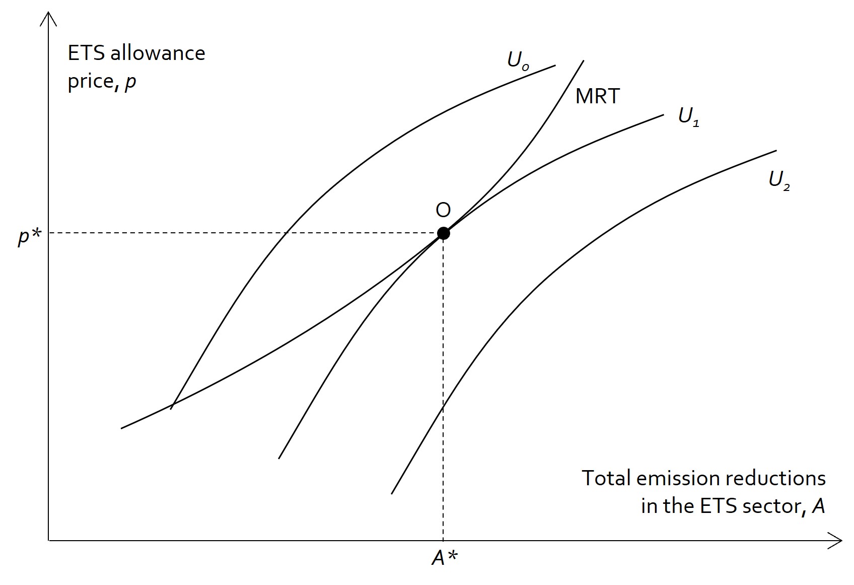
This mechanism is illustrated in Figure 3, in which the MRT (marginal rate of transformation) curve indicates the ETS allowance price p needed to ensure a given amount A of total emission reductions in the ETS sector for the EU as a whole. The MRT curve is upward-sloping since it takes a higher allowance price to induce a larger volume of emission abatement. Moreover, the slope of the MRT curve is increasing, reflecting increasing marginal abatement costs: As the level of abatement increases and the cheaper abatement options are exhausted, it requires a larger increase in the allowance price to reduce emissions by one more tonne.

Figure 3 also includes three ‘indifference curves’ for EU policy makers, each labelled by a U. These indifference curves describe the preferences of policy makers, and each curve corresponds to a given level of policy maker ‘utility’ or policy maker popularity. Ceteris paribus, policy makers become more popular if they can ensure a larger volume of abatement, but they become less popular if the ETS allowance price goes up, since a higher allowance price translates into higher energy prices for households and companies. To maintain a given level of policy maker popularity, a higher allowance price must therefore be accompanied by a higher level of abatement. Hence, the indifference curves are upward-sloping, but the slope decreases as the allowance price goes up, since the marginal welfare loss for energy consumers increases as energy prices increase. An indifference curve located further to the right represents a higher level of utility, since policy makers prefer a higher level of abatement for any given level of the allowance price (and a lower allowance price for any given abatement level). To maximise their utility (popularity), EU policy makers will adjust the ETS allowance supply (and hence the allowance price) so as to realise the point O on the MRT curve where they cannot attain a higher utility, given that the combination of A and p must be located somewhere on the MRT curve. At this optimum point, the slope of the indifference curve equals the slope of the MRT curve.

Figure 3. Political endogeneity of the cap on emission allowance

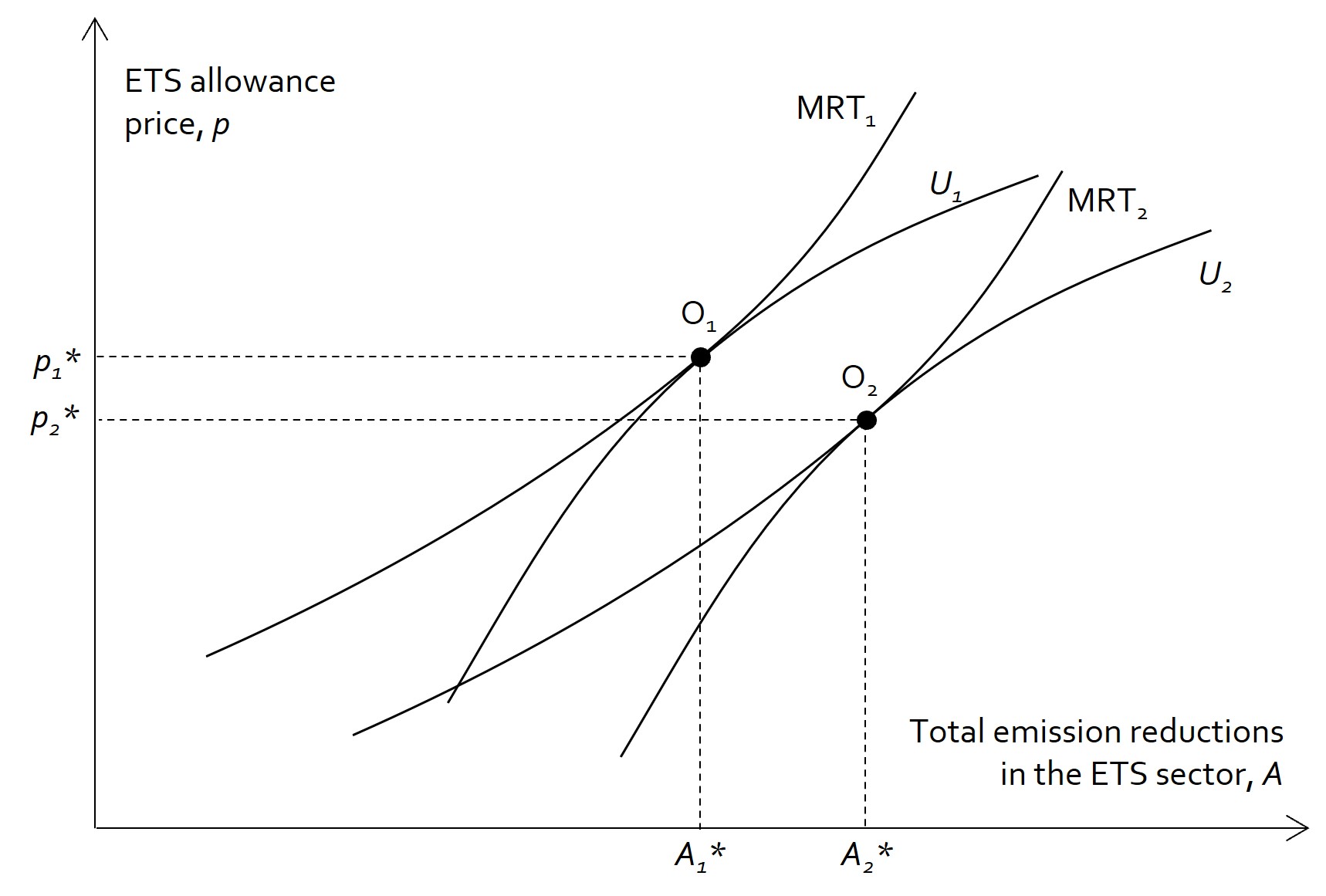
Now suppose that an EU frontrunner country decides to introduce a national carbon tax on top of the ETS allowance price. As the carbon tax induces the country’s emitters to increase their abatement efforts, the MRT curve will shift to the right, since any given allowance price will now be associated with a larger total level of abatement in the EU. As a consequence, the EU’s political economy equilibrium will shift from point 0₁ to point 0₂ in Figure 4, where total abatement in the EU as a whole has increased despite the fall in the allowance price. In Figure 4, we see that the distance from point A₁^∗ to point A₂^∗ is shorter than the rightward horizontal shift of the MRT curve measuring the increase in abatement in the frontrunner country. Therefore, there will be some leakage of emissions from the frontrunner country to the rest of the EU, but the leakage rate will be less than 100%. Appendix A specifies a set of plausible technical conditions which will be sufficient to ensure this result.

Figure 4. Effect of an increase in abatement effort in a single EU member state on the political economy equilibrium of the ETS

The mechanism underlying the increase in total abatement is the following: The rise in carbon taxation in the frontrunner country increases abatement in that country, thereby releasing some ETS allowances which are offered for sale in the allowance market. If the total allowance supply were kept constant, the allowance price would then have to drop to a level that would generate a fall in abatement in the rest of the EU corresponding to the increase in abatement in the frontrunner country (100% leakage). However, since the allowance price has now fallen without generating an increase in total emissions, the trade-off between the desire for a low allowance price and the desire for a strong abatement effort becomes more favourable for EU policy makers. They prefer, therefore, to realise a part of the resulting utility gain in the form of a larger abatement effort and only part of the gain in the form of a lower allowance price. To achieve a fall in total emissions (i.e., an increase in total abatement), EU policy makers must thus decide to cut the total supply of emission allowances.

The graphical analysis above ignores the existence of the Market Stability Reserve. However, the effect of a reserve is easily understood. Its main effect is the automatic cancellation of allowances, but since the EU controls emissions, it can adjust the cap in the light of any MSR cancellations. This leads to two conclusions. First, the MSR does not alter our argument regarding the political endogeneity of the ETS cap, and even though the current ETS rules appear to imply a 100% leakage rate from unilateral national climate policy after 2031, the actual leakage rate is likely to become lower due to the political economy mechanisms described above. Second, the possibility of reducing the ETS cap through the MSR vanishes when we add political endogeneity. Or put differently, both types of endogeneity cannot exist to their full extent at the same time.

We now turn to the second major issue addressed in this paper: What is the optimal unilateral climate policy in an EU frontrunner country? We consider a country which has committed itself to a target for the reduction of total domestic emissions that goes beyond its EU obligations, as Denmark, Finland and Sweden have done, and we assume that this country imposes a carbon tax on all domestic emissions of CO₂e as the main policy instrument to meet its target. In the EU, the Effort Sharing Regulation (ESR) sets national targets for emission reductions from road transport, heating of buildings, agriculture, small industrial installations and waste management. There are also national targets for net greenhouse gas removals in the land use, land use change and forestry (LULUCF) sector, but since emission rights can be transferred between the ESR and LULUCF sectors (with some restrictions), we will treat these as one consolidated sector denoted the ‘non-ETS sector’.

The ‘carbon price’ is the cost to companies and households of emitting an extra tonne of CO₂e. In the non-ETS sector, the carbon price is simply the domestic carbon tax rate. In the ETS sector, the carbon price is the sum of the domestic carbon tax rate and the price of ETS allowances if no credit for the allowance price is granted against the domestic carbon tax. The key policy question is whether or not the domestic carbon price should be the same across the ETS and the non-ETS sector, i.e., whether companies in the ETS sector should receive a 100% credit for the ETS allowance price against the (uniform) domestic carbon tax rate. The conventional answer to this question is “Yes”, since it is believed that a uniform carbon price throughout the economy ensures that the target for domestic emission reduction is met in a cost-effective way. The reason for this is that cost-minimising companies and households will abate their emissions up to the point where their marginal abatement cost equals the carbon price, so through a uniform carbon price, all emitters will end up with the same marginal abatement cost, thereby ensuring that the total abatement cost in the economy as a whole is minimised.

However, in the following, we will show that a uniform domestic carbon price is generally suboptimal in an EU frontrunner country wishing to minimise the total national cost of meeting the target for domestic emission reduction. As will be revealed, the basic reason for this is that emission rights in the ETS sector and in the non-ETS sector can be traded between the domestic country and the rest of the EU, but not necessarily at the same price across the two sectors. Furthermore, the domestic government may worry about carbon leakage, and if the leakage rates differ between the ETS sector and the non-ETS sector – as they probably do, this gives further grounds for differentiating the total carbon price across the two sectors. We illustrate these points graphically below, inspired by the work of Kruse-Andersen and Sørensen (2022b)

Kruse-Andersen and Sørensen (2022b) only account for trade in ETS allowances. Here, we extend their analysis by allowing for trade in emission rights for the non-ETS sector (in Figures 6 and 7).

and building on the formal analysis in Appendix B

Although there is no private market for international trade in emission rights in the non-ETS sector, the EU does allow national governments to engage in bilateral trade in such emission rights (within certain limits). Thus, the government of an EU country may meet part of its obligation to cut emissions from the non-ETS sector by purchasing emission rights allocated to another EU government. For the moment, we will assume that the ambitious EU country does not plan to exploit the opportunity for trade in non-ETS emission rights and that its target for domestic emission reduction is sufficiently strict to ensure that the country’s obligations under the EU Effort Sharing Regulation do not become a binding constraint on domestic climate policy. We also assume, for a start, that the country’s government is not concerned about carbon leakage.

We can illustrate the country’s cost-effective climate policy by means of Figure 5. The distance from A to B along the horizontal axis measures the government’s target for the reduction of total domestic emissions from today until, say, 2030, measured in tonnes of CO₂e. The size of the cut in emissions from the domestic ETS sector is measured from left to right on the horizontal axis, while the reduction of emissions from the non-ETS sector is measured from right to left. The vertical axes measure the marginal costs of abating emissions from the two sectors, and the graphs denoted MAC^ETS and MAC^Non-ETS indicate the marginal abatement costs in the ETS and the non-ETS sector, respectively. Since cost-minimising companies and households will exploit the cheaper options for emission reduction before transitioning to the more expensive options, the marginal abatement costs are higher the larger the cut in emissions. For simplicity, we assume that the marginal abatement cost curves are linear. In practice, they are likely to be convex towards the origin, but this will not invalidate the qualitative conclusions from our analysis.

According to conventional wisdom, a cost-effective national climate policy requires that the total carbon price be equalised across the ETS and the non-ETS sector. Cost-minimising agents will then reduce their emissions up to the point where their marginal abatement costs equal the common carbon price so that the economy’s overall abatement costs are minimised. In Figure 5, this situation is attained at point E which would thus seem to represent the optimal allocation of emission cuts between the ETS and the non-ETS sector. However, this analysis neglects that for each tonne of emission reduction in the ETS sector, the companies in that sector save a cost equal to the price of an ETS emission allowance, denoted by p^q in Figure 5. When a domestic ETS sector company needs one less emission allowance, it can sell the allowance in the ETS market for allowances, thereby earning an amount p^q. Since this amount is a transfer from the rest of the EU economy to the domestic economy, it represents a corresponding reduction in the total domestic marginal social cost of cutting emissions from the domestic ETS sector.

Figure 5. Cost-effective allocation of abatement effort when emission rights for the non-ETS sector are not traded

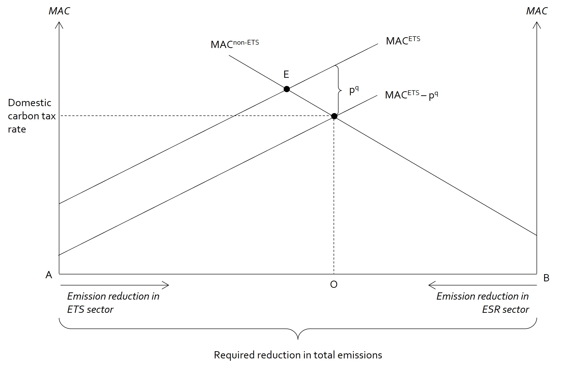
Hence the net marginal social abatement cost in the ETS sector is given by the graph denoted MAC^ETS-p^q in Figure 5. From a national viewpoint, a cost-effective allocation of emission cuts between the two sectors is attained when the net marginal social abatement cost in the ETS sector equals the marginal abatement cost in the non-ETS sector. In Figure 5, this optimum is realised when the allocation of emission reductions corresponds to point O on the horizontal axis. To implement this allocation, the domestic carbon tax rate must be set at a level corresponding to the marginal abatement cost in the non-ETS sector at point O. At that point, the gross marginal abatement cost MAC^ETS in the ETS sector exceeds the marginal abatement cost in the non-ETS sector by the amount p^q corresponding to the ETS allowance price, but since an individual ETS company, as well as the domestic economy as a whole, saves the expenditure p^q for each tonne of emission cuts in the ETS sector, the net marginal abatement cost in that sector equals the marginal abatement cost in the non-ETS sector at the optimum point O.

In summary, when there is no trade in emission rights for the non-ETS sector and the government is not worried about carbon leakage, a nationally optimal allocation of emission cuts requires that companies in the ETS sector be granted no credit at all for the ETS allowance price against their domestic carbon tax bill: Under the optimal climate policy, the total carbon price in the ETS sector exceeds the carbon price in the non-ETS sector (the uniform domestic carbon tax rate) by an amount equal to the ETS allowance price. This is “Model 1” for a domestic carbon tax scheme proposed by the Danish government’s Expert Group on Green Tax Reform (2022).

Matters become different if the domestic government adopts a more pragmatic version of the target for domestic emission reduction, allowing itself to purchase emission rights for the non-ETS sector from other EU governments if reducing domestic emissions to the extent required by the Effort Sharing Regulation proves overly expensive, and by selling non-ETS emission rights to other EU member states if the ESR is not a binding constraint on the planned domestic climate policy. This situation is depicted in Figure 6, which assumes that emission rights for the non-ETS sector can be purchased at the price p^N per tonne of CO₂e. By an analogous reasoning to the one underlying Figure 5, the net marginal social abatement cost in the non-ETS sector is now given by the curve MAC^Non-ETS - p^N in Figure 6, since the government (and domestic society) saves an expenditure equal to the price of foreign non-ETS emission rights for each tonne of domestic non-ETS emission reduction – money that would have had to be transferred to another EU government if the domestic emission reduction had not been undertaken.

The net marginal social abatement cost in the non-ETS sector would still be given by the curve MAC^Non-ETS - p^N in Figure 6 if the domestic government had a surplus of non-ETS emission rights it could sell abroad, since an extra tonne of domestic non-ETS emission reduction would then enable the government to sell one more unit of emission rights to a foreign government, thereby generating an extra transfer p^N to the domestic economy.

The optimal allocation of emission cuts between the ETS and the non-ETS sector is now given by the point of intersection of the two curves MAC^ETS - p^q and MAC^Non-ETS - p^N where the net marginal social abatement costs are equalised across sectors. To implement this allocation O, the domestic carbon tax rate must be set at the level indicated on the left vertical axis in Figure 6.

Figure 6. Cost-effective allocation of abatement effort when emission rights for the non-ETS sector are traded

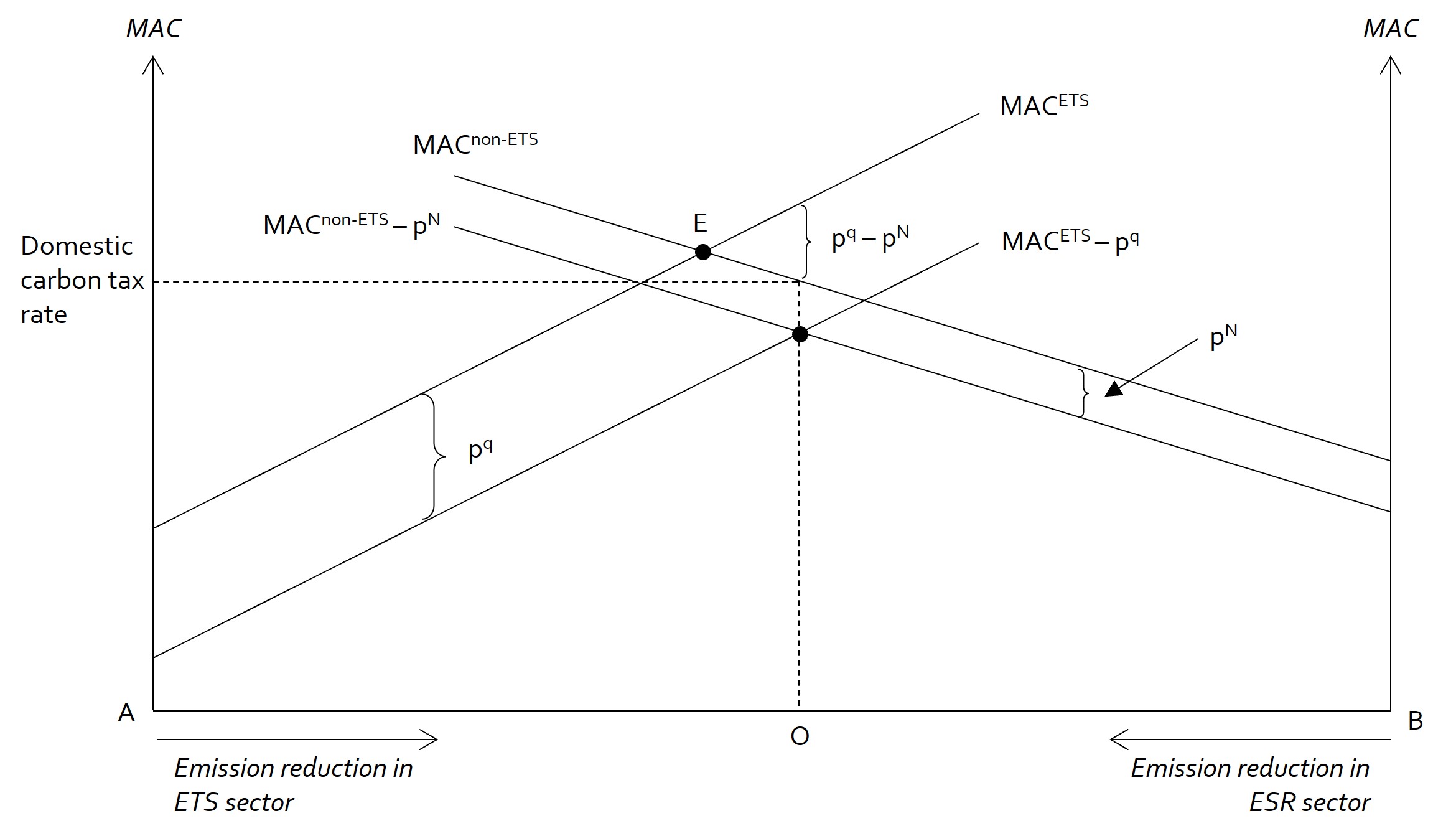
Note that since emission rights for the non-ETS sector are not traded privately but only among governments, cost-minimising non-ETS emitters will abate up to the point where their private marginal abatement cost MAC^Non-ETS equals the domestic carbon tax rate. When the carbon tax rate is set at the level illustrated in Figure 6, emitters in the non-ETS sector are therefore induced to undertake the optimal amount of abatement BO. In this optimum, the gross marginal abatement costs in the two sectors (MAC^ETSand MAC^Non-ETS) are seen to differ by an amount equal to the difference between the ETS allowance price and the price of non-ETS emission rights. In Figure 6, we assume that the former price is higher than the latter. We see that now the total carbon price in the ETS sector should only exceed the domestic carbon tax rate by the amount p^q - p^N. This means that domestic ETS companies should receive a partial credit for the ETS allowance price equal to the amount p^N per tonne of CO₂e against their domestic carbon tax bill to ensure a total carbon price for ETS companies equal to the carbon tax rate + p^q - p^N consistent with the optimal allocation O in Figure 6.

If the price of non-ETS emission rights were to exceed the ETS allowance price, the optimal allocation of emission cuts would lie to the left of point E in Figure 6 rather than to the right of this point. In the interesting special case where the price of emission rights is the same across sectors (p^q = p^N), it is clear from Figure 6 that the optimal allocation would be at point E, consistent with the conventional recommendation that gross marginal abatement costs be equalised across sectors, since in this particular case the net marginal social abatement costs would also be equalised. In this case, ETS companies should receive a full credit for the allowance price against the domestic carbon tax. However, since the markets for ETS and non-ETS emission rights are not integrated in the EU, the prices of the two types of emission rights would only align by pure coincidence.

We have so far assumed that the domestic government is not concerned about carbon leakage. However, suppose that when emissions from the domestic ETS sector fall by 1 tonne of CO₂e, emissions from foreign countries increase by a tonnes (on average) via carbon leakage operating through the mechanics of the ETS described in Section 2. Suppose further that the domestic government worries about leakage (because it is concerned about the impact of domestic policy on the global climate) and therefore assigns a social cost c to a tonne of CO₂e emitted abroad. The marginal social cost of the leakage from the ETS sector (MSCL^ETS ) generated by a 1 tonne cut in emissions from the sector is then equal to a∙c, where a is the leakage rate. This leakage cost is part of the total net marginal social cost of abatement in the ETS sector, which now becomes MAC^ETS - p^q + MSCL^ETS, as illustrated in Figure 7 where we assume that MSCL^ETS < p^q (which is not, however, important for our qualitative reasoning). Similarly, if the leakage rate in the non-ETS sector is b, the marginal social cost of leakage from that sector is MSCL^Non-ETS = b ∙ c, and the total net marginal social cost of abatement in the non-ETS sector is MAC^Non-ETS - p^N + MSCL^Non-ETS, as shown in Figure 7 where we also assume, specifically, that MSCL^Non-ETS < p^N.

Figure 7. Cost-effective allocation of abatement effort when emission rights are traded and carbon leakage is socially costly

The cost-effective domestic allocation of emission cuts is given at point O in Figure 7, where the curves for the net marginal social cost of abatement in the two sectors intersect. This allocation minimises the total social cost of meeting the target for domestic emission reduction, accounting for the social costs of carbon leakage as well as for trade in emission rights in both sectors. As the figure is drawn, the optimal allocation lies to the right of point E, implying that society should accept a higher gross marginal abatement cost in the ETS sector than in the non-ETS sector. This means that ETS companies should still only receive a partial credit for the ETS allowance price against the domestic carbon tax. More precisely, the tax credit should be equal to p^N + MSCL^ETS - MSCL^Non-ETS per tonne of CO₂e emitted from the ETS sector to implement the optimal allocation O in Figure 7.

To see this, note that a cost-minimising ETS emitter will abate up to the point where MAC^ETC = τ + p^q - κ, where τ is the domestic carbon tax rate, and κ is the carbon tax credit. Moreover, cost-minimising non-ETS emitters will abate until MAC^Non-ETC = τ. Hence MAC^ETC = MAC^Non-ETC + p^q - κ. Therefore, if the tax credit is κ = p^N + MSCL^ETS - MSCL^Non-ETS, it follows that MAC^ETC - p^q + MSCL^ETS = MAC^Non-ETC - p^N + MSCL^Non-ETS which is exactly the condition for an optimal allocation of abatement effort across the two sectors, so a tax credit of this magnitude would lead to the optimal allocation.

In other words, the larger the rate of carbon leakage (and consequently the higher the marginal social cost of leakage) in the ETS sector relative to the leakage rate in the non-ETS sector, the larger the optimal tax credit for (part of) the ETS allowance price becomes, which is intuitive.

With a different combination of allowance prices and marginal social leakage costs, the optimal allocation could lie to the left of point E, in which case ETS companies should be granted a credit greater than 100% for the ETS allowance price or, alternatively, should receive a 100% credit for the allowance price and pay a lower rate of carbon tax than emitters in the non-ETS sector.

Note that the leakage rate a in the ETS sector also measures the fall in foreign emissions generated by a one-tonne increase in the excess domestic demand for ETS allowances, i.e., a measures the fall in foreign emissions that would materialise if the domestic government decided to purchase one ETS emission allowance and withdraw it from the market. Hence, the amount MSCL^ETS = a∙c also measures the marginal social benefit from the government’s purchase of an ETS allowance. If this marginal benefit exceeds the allowance price p^q, the government could generate a domestic welfare gain by purchasing ETS allowances until its marginal willingness to pay for foreign emission cuts (i.e., c) falls to a level where a∙c becomes equal to the allowance price. On the other hand, if MSCL^ETS = a∙c is initially lower than the allowance price, the government should sell emission allowances in the ETS market (so long as it holds such allowances allocated to it by the EU) until MSCL^ETS and the allowance price are driven into line. Theoretically, it could thus be argued that a rational government should intervene in the ETS allowance market to ensure that MSCL^ETS = p^q. If a similar arbitrage behaviour in the non-ETS sector were to ensure that MSCL^Non-ETS = p^N, the optimal allocation of emission reductions would be given by point E in Figure 7, again validating the conventional recommendation that gross marginal abatement costs be equalised across sectors. Once more, this would require a 100% credit for the ETS allowance price against the domestic carbon tax bill of ETS companies.

In practice, governments rarely behave in such a rational manner, and even if they tried to do so, the lack of an integrated and liquid market for emission rights in the non-ETS sector would probably prevent an equalisation of the marginal social cost of leakage and the emission allowance price in that sector.

Realistically, we would, therefore, expect the cost-effective allocation of emission reductions to deviate from point E in Figure 7. This, in turn, implies that the optimal domestic carbon tax credit for the ETS allowance price will deviate from 100%, i.e., that the optimal total carbon prices in the ETS sector and the non-ETS sector will differ from each other.

The analysis in this section can be summarised as follows: The marginal social cost of abatement in an economic sector includes the technical marginal abatement cost plus the marginal social cost of carbon leakage from the sector minus the international price of emission rights in the sector. The criterion for an optimal unilateral climate policy is that the marginal social costs of abatement should be equalised across sectors. This means that a uniform carbon price across sectors is not necessarily the optimal setting. If the domestic government does not worry about carbon leakage, a uniform carbon price is cost-effective only if the international price of emission rights is the same in the ETS and the non-ETS sector. If the government is concerned about leakage, a uniform carbon price for all private emitters is only optimal if the rates of carbon leakage as well as the prices of emission rights are the same across the two sectors, which is unlikely to be the case.

A relatively high carbon leakage rate and a relatively low international price of emission rights in a given sector work in favour of having a relatively low total carbon price in that sector. A priori this theoretical insight does not tell us unambiguously whether the ETS sector should have a higher or a lower carbon price than the non-ETS sector. However, we found that if the government cannot or does not wish to trade emission rights for the non-ETS sector and is relatively unconcerned about carbon leakage, the total carbon price in the ETS sector should generally exceed the carbon tax rate levied on the non-ETS sector, i.e., some amount of domestic carbon tax should be imposed on the ETS sector on top of the ETS allowance price. The reason is that the allowance price makes it more expensive for society to emit CO₂e from the ETS sector. In effect, the EU co-finances a part of the domestic cost of abating emissions from the ETS sector since the domestic economy saves the expense on an ETS allowance when emissions from that sector are cut by one tonne. Ceteris paribus, this makes it more attractive to reduce emissions from the ETS sector and consequently warrants a higher carbon price in the sector.

The policy recommendations above depend to a large extent on the specific target for domestic climate policy. This can be illustrated by comparing climate policy targets in Norway and Denmark. According to the Norwegian Climate Act, the total domestic CO₂e emissions in Norway must be cut by 55% by 2030 compared to 1990, to live up to the country’s commitment under the Paris Agreement. Norway co-operates with the EU on climate policy and participates in the ETS even though Norway is not a member of the EU. The Norwegian ETS sector’s contribution to the fulfilment of Norway’s obligations under the Kyoto Protocol, which preceded the Paris Agreement, was determined in negotiations with the EU. It was decided that Norway should be given a credit for emission reductions in the ETS sector corresponding to the reduction over time in the amount of ETS allowances allocated to the country under the ETS

The amount of ETS allowances allocated to Norway was defined as the amount by which the total issue of ETS allowances was increased as a consequence of the country’s participation in the ETS.

. In other words, under the Kyoto Protocol in effect until 2020, the contribution of the Norwegian ETS sector to fulfilment of the country’s target for total emission reductions did not depend on the actual emissions from the sector but rather on the politically determined quantity of ETS allowances allocated to Norway by the EU.

The contribution of the Norwegian ETS sector to the country’s 2030 climate target has yet to be negotiated with the EU, but it is expected that it will be determined in much the same way as under the Kyoto Protocol. In such a situation where a cut in the actual emissions from the ETS sector does not contribute to the fulfilment of the country’s national climate policy target, there is no case for imposing a domestic carbon tax in the ETS sector on top of the allowance price. Instead, the carbon tax should only apply to the non-ETS sector.

By contrast, according to the Danish Climate Act, which requires a 70% cut in total domestic emissions by 2030 relative to 1990, the ETS sector’s contribution to fulfilling this target is measured by the reduction of actual emissions from the sector, as assumed in our analysis above. Under such a specification of the policy target, the carbon price for the ETS sector should, in fact, include some amount of domestic carbon taxation when policy makers strive to secure domestic cost-effectiveness, as we have seen.

This conclusion assumes that the goal of domestic climate policy is to maximise national welfare rather than securing cost-effectiveness throughout the EU as a whole. This approach could be defended by the fact that a frontrunner country voluntarily incurs higher abatement costs than those required for fulfilment of its obligations towards the EU, and so it may legitimately seek to minimise the national cost of moving ahead of the EU. It can also be argued that a frontrunner country does not necessarily provide a viable example to other countries if the frontrunner mainly achieves its ambitious target for emissions reduction by forcing the production of CO₂e-intensive goods abroad rather than by reducing emissions per unit of domestic output. From this perspective, the frontrunner’s carbon tax scheme should account for the risk of carbon leakage in line with the policy design illustrated in Figure 7.

On the other hand, one could adopt the “Kantian” approach that a frontrunner country seeking to lead by example should pursue a climate policy similar to one it would like adopted by the whole of the EU. Presumably, this would be a policy securing a cost-effective abatement of total EU emissions, i.e., a climate policy ensuring an equalisation of the total carbon price between the ETS and the non-ETS sector. Such an approach to national climate policy in an EU frontrunner country should not discriminate between the two sectors.

The choice between these two approaches is obviously a normative issue to be decided, in the end, by policy makers.

In the introduction, we mentioned some reasons why the Nordic countries might want to act as frontrunners in EU climate policy. We then challenged the conventional wisdom on the design of unilateral climate policy on two fronts.

According to the conventional view, unilateral action to reduce emissions from the ETS sector in a single EU country makes little sense, since the rate of carbon leakage to other EU countries will be 100%, at least in the long term, where the total cap on emissions is likely to be binding. However, in both the short and medium term, a unilateral cut in emissions from a country’s ETS sector will, in fact, permanently reduce the concentration of CO₂e in the atmosphere due to the intricate mechanics of the Market Stability Reserve (MSR) in the ETS, although the precise overall effect on total emissions is difficult to predict. More fundamentally, we argued that the total amount of emission allowances issued over the long term is likely to be endogenous, as EU policy makers trade off their desire to control the quantity of emissions against their desire to avoid excessive fluctuations in the allowance price. Under such a policy setting, a unilateral member state policy that reduces emissions from the ETS sector, thereby creating a greater allowance surplus, will sooner or later induce a cut in the total allowance supply. The introduction and recent reforms of the MSR suggest that such political dynamics are, in fact, at play in the EU, implying that unilateral climate policy aimed at the ETS sector does have a permanent climate impact.

Another conventional view is that a cost-effective way of meeting a target for reduction of domestic greenhouse gas emissions is to implement a uniform carbon price across all sectors of the economy. Under such a policy, companies in the ETS sector would be granted a 100% credit for expenses on ETS allowances set against their domestic carbon tax bill. We saw that such a policy could be defended under a “Kantian” policy approach, but if the aim of domestic climate policy is to maximise national welfare, we found that a uniform carbon price is only cost-effective under rather special circumstances which are unlikely to prevail. Instead, we showed that the carbon price should be differentiated between the ETS and the non-ETS sector according to differences in the international prices of emission rights and differences in carbon leakage rates (when carbon leakage is a concern for the government).

In practice, designing the optimal unilateral carbon tax scheme for an EU frontrunner country will be difficult due to uncertainties surrounding the future price of emission rights and carbon leakage rates in the different sectors. This could present an argument for restricting the use of reduced carbon prices to a few subsectors where the risk of leakage is likely to be high.

Finally, we should note that rather than addressing carbon leakage via tax credits and/or reduced carbon tax rates for (sub)sectors exposed to leakage, the government could, in principle, grant an output subsidy to such sectors, combined with a consumption tax on similar imported goods, differentiated according to their carbon content.

For a formal analysis of the various instruments to counter carbon leakage, see Kruse-Andersen and Sørensen (2022a).

In this paper, we have ignored such national policy instruments as they may be incompatible with EU law and difficult to administer.

Beck, U., & Kruse-Andersen, P. K. (2020). Endogenizing the Cap in a Cap-and-Trade System: Assessing the Agreement on EU ETS Phase 4, Environmental and Resource Economics, 77, 781–811.

Expert Group on Green Tax Reform. (2022). Grøn skattereform – Første delrapport. [Green Tax Reform – Initial Report]. Copenhagen, February 2022, Retrieved from (https://www.skm.dk/media/10993/groen-skattereform-foerste-delrapport-tilgaengelig.pdf)

Gerlagh, R., Heijmans., R. J. R. K., & Rosendahl, K. E. (2021). An endogenous emissions cap produces a green paradox. Economic Policy, 36(107), 485–522.

Greaker, M., Golombek, R., & Hoel, M. (2019). Global impact of national climate policy in the Nordic countries. Nordic Economic Policy Review 2019, 157-202.

Kant, I. (1993). Grounding for the Metaphysics of Morals. (J.W. Ellington translation). Hackett Publishing Company. (Original work published 1785).

Kruse-Andersen, P.K., & Sørensen, P.B. (2022a). Optimal energy taxes and subsidies under a cost-effective unilateral climate policy: Addressing carbon leakage. Energy Economics, 109, May 2022, 105928.

Kruse-Andersen, P.K., & Sørensen P.B. (2022b). Optimal climate policy in EU frontrunner countries: coordinating with the EU ETS and addressing leakage. Climate Policy, November 2022 (https://doi.org/10.1080/14693062.2022.2145259).

Perino, G. (2018). New EU ETS Phase 4 rules temporarily puncture waterbed. Nature Climate Change, 8 (4), 262-270.

Silbye, F., & Sørensen, P. B. (2019). National Climate Policies and the European Emissions Trading System, Nordic Economic Policy Review, 2019(12), 63-101.

Stavins, R. N. (2019). Carbon Taxes vs. Cap and Trade: Theory and Practice, Harvard Project on Climate Agreements, Discussion Paper ES 19–9.

In this appendix, we set up the political economy model for the determination of the supply of ETS emissions allowances which underlies Figures 3 and 4. We assume that the preferences of EU policy makers are given by a ‘utility function’ of the following form,

$$ U=U(A,p), $$ (A.1)

$$ U_A\equiv\frac{\partial U}{\partial A}>0, $$ $$ U_{AA}\equiv\frac{\partial^2U}{\left(\partial A\right)^2}<0, $$ $$ U_p\equiv\frac{\partial U}{\partial p}<0, $$
$$ U_{pp}\equiv\frac{\partial^2U}{\left(\partial p\right)^2} $$ $$ <0, $$ $$ U_{Ap}=U_{pA}\equiv\frac{\partial^2U}{\partial A\partial p}=\frac{\partial^2U}{\partial p\partial A}\le0, $$

where 𝐴 is the total volume of abatement of CO₂ emissions from the EU ETS sector, and 𝑝 is the price of ETS emission allowances. The assumption 𝑈_𝐴 > 0 reflects that, ceteris paribus, EU policy makers are more popular the larger the cut in ETS emissions they manage to secure, but since 𝑈_𝐴𝐴 < 0, the marginal popularity gain from emission reduction decreases with the level of abatement. The assumptions 𝑈_𝑝 < 0 and 𝑈_𝑝𝑝 < 0 mean that, ceteris paribus, EU policy makers lose popularity when the ETS allowance price goes up and that the marginal loss of popularity increases with the allowance price level. These assumptions reflect that a higher allowance price translates into higher energy prices which are unpopular with voters and industry. The final technical assumption 𝑈_𝐴𝑝 = 𝑈_𝑝𝐴 ≤ 0 is sufficient (but not necessary) to ensure that the indifference curves in Figures 3 and 4 are indeed concave, as intuition suggests. The utility function (A.1) should be thought of as a weighted average of the preferences of individual EU member states, where the weights depend on the distribution of voting rights and bargaining power.

The total abatement in the ETS sector is the sum of abatement undertaken by a frontrunner EU member state, 𝑔(𝑝 + τ), where τ is the frontrunner country’s domestic carbon tax rate which adds to the total domestic carbon price 𝑝 + τ, and the abatement implemented in the rest of the EU, 𝑓(𝑝). A higher carbon price induces greater abatement efforts, but at a decreasing rate since marginal abatement costs increase with the level of abatement. Hence,

$$ A=\overbrace{g\left(p+\tau\right)}^{\text{Abatement in front runner country}}+\overbrace{f\left(p\right)}^{\text{Abatement in the rest of the EU}}, $$
g^'>0, g^{^{}\prime\prime}<0, f^'>0, f^{^{}\prime\prime}<0. (A.2)

In the absence of the ETS and national climate policies, the total emissions from the ETS sector would equal the business-as-usual level 𝐸₀ which we treat as exogenous, but under the ETS and the national climate policy in the frontrunner country, actual emissions become 𝐸₀ - 𝑔(𝑝 + τ) − 𝑓(𝑝). The total supply of ETS emission allowances is 𝑆̅, so the equilibrium allowance price must satisfy the market equilibrium condition

E_0-g(p+\tau)-f(p)=\overline{S}. (A.3)

Equation (A.3) may be solved for the equilibrium allowance price to give a price function of the form

\frac{-g^'}{f^'+g^'}<0. (A.4)

Inserting (A.2) and (A.4) in (A.1), we get

U=U(f\left(p\left(\overline{S},\tau\right)\right)+g(p\left(\overline{S},\tau\right)+\tau),p\left(\overline{S},\tau)\right). (A.5)

Rational EU policy makers will choose the supply of ETS emission allowances so as to maximise the utility function (A.5). The first-order condition for maximisation is

-\frac{U_A}{U_p}=\frac{1}{f^{\prime}+g^{\prime}}.  (A.6)

Equation (A.6) is the formal characterisation of the optimum point O in Figure 3 where the slope of the indifference curve 𝑈₁ (the left-hand side of (A.6)) equals the slope of the MRT curve (the right-hand side of (A.6)). The optimum condition (A.6) can be written in the form

 

[f^{\prime}(p(\overline{S},\tau))+g^{\prime}(p(\overline{S},\tau)+\tau)]U_A(f(p\left(\overline{S},\tau\right)) $$ +g(p\left(\overline{S},\tau\right)+\tau),p(\overline{S},\tau)) $$

+U_p(f(p\left(\overline{S},\tau)\right)+g(p\left(\overline{S},\tau\right)+\tau),p\left(\overline{S},\tau\right))=0. (A.7)

Equation (A.7) defines the total ETS allowance supply \overline{S}as an implicit function of the frontrunner country’s carbon tax rate τ. If \frac{d\overline{S}}{d\tau}<0, the introduction of a national carbon tax in the frontrunner country will induce a fall in the allowance supply, thereby reducing total EU emissions. By implicit differentiation of (A.7) and use of the results in (A.4), we find after some manipulations that

\frac{\partial\overline{S}}{\partial\tau}=-\lbrace{\frac{g^{\prime}[U_{pp}+(f^'+g^{\prime})U_{Ap}+U_Af^{\prime}\frac{f^{\doubleprime}}{f^{\prime}}-\frac{g^{\doubleprime}}{g^{\prime}})]}{U_{pp}+U_A(f^{^{\prime\prime}}+g^{\doubleprime})+U_{AA}(f^'+g^{\prime})^2+2(f^'+g^{\prime})U_{Ap})}\rbrace} (A.8)

As a benchmark, suppose the frontrunner country and the rest of the EU have access to the same abatement technologies so that the slopes of their marginal abatement cost curves are identical. For example, this will be the case if

f(p)=ap^{\alpha},\quadg(p+\tau)=b(p+\tau)^{\alpha},\quad$$ 0<\alpha<1, $$ (A.9)

where 𝑎 and 𝑏 are positive scalars. If the frontrunner country starts out from an initial carbon tax rate of zero, it follows from (A.9) that

\frac{f^{\doubleprime}}{f^{\prime}}-\frac{g^{\doubleprime}}{g^'}=\frac{a\alpha(\alpha-1)p^{\alpha-2}}{a\alpha p^{\alpha-1}}-\frac{b\alpha(\alpha-1)p^{\alpha-2}}{b\alpha p^{\alpha-1}}=\frac{\alpha-1}{p}-\frac{\alpha-1}{p}=0. (A.10)

Given the properties of the utility function specified in (A.1), we see from (A.8) that the result in (A.10) is a sufficient (but not a necessary) condition to ensure that \frac{d\overline{S}}{d\tau}<0. Hence, it seems safe to conclude that, under plausible conditions, the introduction of a national carbon tax on top of the ETS allowance price in an EU frontrunner country will indeed reduce total EU emissions by inducing a cut in the total allowance supply, as illustrated in Figure 4.

This appendix describes the formal analysis underlying Figures 5 through 7 in section 3. We use the following notation where all variables refer to the domestic economy:

TC= total social cost

TAC^{ETS}= total abatement cost in the ETS sector

TAC^{non-ETS}= total abatement cost in the non-ETS sector

A^{ETS} emission reduction in the ETS sector

A^{non-ETS}= emission reduction in the non-ETS sector

\overline{A}= total required domestic emission reduction (exogenous)

E_0^{ETS}= business-as-usual emissions from the ETS sector (exogenous)

E_0^{non-ETS}= business-as-usual emissions from the non-ETS sector (exogenous)

\overline{E}^{ETS}= ETS emission allowances allocated to the country (exogenous)

\overline{E}^{non-ETS}= emissions from the country’s non-ETS sector allowed by EU regulation (exogenous)

a^{ETS}= rate of carbon leakage from the ETS sector (exogenous)

a^{}^{non-ETS}= rate of carbon leakage from the non-ETS sector (exogenous)

c= domestic willingness to pay for a 1 tonne cut in foreign emissions (unit social cost of leakage, exogenous)

We assume that the social planner wishes to minimise the total national social costs associated with the use of fossil fuel and other inputs generating greenhouse gas emissions. These costs include abatement costs that depend on the levels of abatement, expenses on the purchase of emission rights (since these expenses represent a transfer to the rest of the EU), and the costs of carbon leakage that depend on leakage rates and on the government’s willingness to pay for a reduction in foreign emissions (𝑐). Hence, we have

 

$$ \underbrace{c\cdot\left(\right.a^{ETS}\cdot A^{ETS}+a^{non-ETS}\cdot A^{non-ETS})}_{\text{Cost of carbon leakage}} $$ (B.1)

where we assume that marginal abatements costs (𝑀𝐴𝐶) are positive and increasing in the level of abatement in both sectors: 

$$ MAC^{Non-ETS}\equiv $$ $$ \frac{dTAC^{Non-ETS}}{dA^{Non-ETS}}>0,\quad $$$$ \frac{d^2TAC^{Non-ETS}}{(dA^{Non-ETS})^2}>0. $$ (B.2)

The social planner chooses the abatement levels 𝐴^𝐸𝑇𝑆 and 𝐴^{𝑁𝑜𝑛-𝐸𝑇𝑆} in the two sectors of the economy so as to minimise the total social cost given by (B.1) subject to the constraint that total abatement is sufficient to meet the target 𝐴̅ for reduction of the total emissions from domestic territory, that is, 

A^{ETS}+A^{Non-ETS}=\overline{A} (B.3)

Solving (B.3) for 𝐴^{𝑁𝑜𝑛-𝐸𝑇𝑆} and inserting the result in (B.1), we can write the total social cost as a function of 𝐴^𝐸𝑇𝑆 only. Doing this, taking the first derivative of the social cost function, and using the definitions of marginal abatement costs stated in (B.2), we obtain the following first-order condition for the optimal abatement effort in the ETS sector:

$$ \overbrace{MAC^{ETS}-p^q+MSCL^{ETS}}^{\text{Net marginal social cost of abatement in ETS sector}} $$$$ =\overbrace{MAC^{Non-ETS}-p^N+MSCL^{non-ETS},}^{\text{Net marginal social cost of abatement in non-ETS sector}} $$  (B.4)

where 𝑀𝑆𝐶𝐿^𝐸𝑇𝑆 ≡ 𝑐 ∙ 𝑎^𝐸𝑇𝑆 and 𝑀𝑆𝐶𝐿^{𝑛𝑜𝑛-𝐸𝑇𝑆} ≡ 𝑐 ∙ 𝑎^{𝑛𝑜𝑛-𝐸𝑇𝑆} are the marginal social costs of leakage in the two sectors. According to (B.4), the cost-effective allocation of abatement effort between the ETS and the non-ETS sector ensures that the net marginal social costs of abatement are equalised across sectors. If the social planner is indifferent to leakage and does not wish to exploit the opportunity for trade in non-ETS emission rights, we have 𝑐 = 𝑝^𝑁 = 0. The optimum determined by (B.4) then corresponds to point 𝑂 on the horizontal axis of Figure 5. When the social planner does exploit the opportunity for trade in non-ETS emission rights but does not care about leakage, we merely have 𝑐 = 0, in which case condition (B.4) gives the optimum point 𝑂 on the horizontal axis of Figure 6. In the scenario where the social planner is concerned about leakage and is willing to engage in trade in emission rights in both sectors, (B.4) identifies the optimum point 𝑂 on the horizontal axis of Figure 7.