Nordic Economic Policy Review 2023

David von Below, Björn Carlén, Svante Mandell and Vincent Otto

Sweden has long supported a more ambitious domestic climate policy than that required by the EU, providing strong incentives for some abatement options (e.g., switching to biofuels or electricity in transport) while other activities have faced a relatively low carbon pricing regime. The Fit for 55 package reduces this ambitions gap. This leads to the question: should Sweden continue to go it alone or harmonise its domestic policy with that of the EU? We use a computable general equilibrium model to assess the cost savings accruing to Sweden from introducing a more uniform domestic climate policy and trading emission-quota units with other member states. The results indicate that such a policy shift would be welfare-enhancing. The analysis does not capture any losses to Sweden by being less of a forerunner (e.g., smaller demonstration effects). An EU-wide cost-benefit analysis of the policy reform would also consider the trade gains accruing to the countries that sell emission-quota units to Sweden.

Keywords: Cost-effective climate policy, international emissions trading, general equilibrium analysis.

JEL codes: C68, Q54, Q58.

The EU has adopted a climate law (‘European Climate Law’; Regulation (EU) 2021/1119, 2021 ) stating that the Union must become climate neutral by 2050 and that its net greenhouse-gas emissions by 2030 should be at least 55% less than those in 1990. To reach these new targets, the European Union’s (EU) climate policy is being revised. This process started when the EU commission released its proposal, Fit for 55, in June 2021.

This paper addresses Sweden’s climate policy in the light of the proposed revisions in Fit for 55. Sweden has long conducted a national climate policy that, by some margin, has been more stringent than that required by the EU. The reasoning behind this approach has been that Sweden should act as a forerunner, providing an example for others to follow. However, based on the proposals put forward in the Fit for 55, the EU is rapidly catching up. For instance, according to the programme, Sweden is obliged to reduce its so-called ESR

ESR is short for Effort Sharing Regulation, which distributes tradable emission quotas among member states. Currently the ESR sector includes non-energy-intensive industries, buildings, road transports, agriculture and small heat and power producers.

emissions in 2030 by 50% relative to 2005, either by domestic actions or by buying emission-quota units from other member states – the Swedish national target corresponds to a domestic reduction of at least 52%. In other respects, in particular, the net uptake of carbon dioxide (CO₂) in forests and land, the proposed EU targets for Sweden are more stringent than Sweden’s national policy aims.

There may be good reasons for Sweden to act as a forerunner. However, there are also costs involved. Given the decreasing margin between Swedish national climate policy and that required by the EU, it might be appropriate to re-evaluate the forerunner strategy. In this paper, we focus on the cost side of the chosen approach. Whether Sweden should only adhere to EU requirements, retain its current forerunner strategy, or opt for even more stringent national targets is for politicians to decide. However, as part of this decision, a thorough discussion of the costs associated with different choices may prove instructive.

The analysis presented below starts with a discussion in which we identify the additional costs that Swedish climate policy imposes on Swedish households. Thereafter we use a computable general equilibrium model of the Swedish economy – EMEC

Environmental Medium-term Economic model.

– to assess the magnitude of these additional costs. The model captures economic activity in Sweden while keeping track of greenhouse-gas emissions. All major climate-policy instruments currently in use in Sweden are explicitly modelled. We use the model to compare the outcome in 2030 under the national climate targets and the policy instruments currently applied to reach them to a situation where Sweden reaches the same reduction of its net emissions in other ways, either by means of different policy instruments or by means of international emissions trading. The difference can be measured in terms of GDP, fuel prices and several other measures that may be of interest.

The paper is organised as follows. The next section provides a brief introduction to the EU’s climate policy framework and the proposals in Fit for 55. It also contains a discussion of the flexibilities that the EU’s climate policy provides. Section 3 details current Swedish climate policy and a formal discussion regarding cost effectiveness. Section 4 introduces EMEC. Section 5 presents a series of model results to illustrate the different policy scenarios’ outcomes. Section 6 concludes.

The European Climate Law (adopted in April 2021) states that the EU must become climate neutral by 2050. The law also includes an interim target for 2030 stating that the Union’s net greenhouse-gas emissions must be reduced by at least 55% compared to 1990 levels. The EU Commission has put forward a series of legislative proposals aimed at reaching these goals. The Commission’s proposal, known as the Fit for 55 package, revises all relevant policy instruments and suggests some new ones. The package strengthens the ambitions of the EU emission trading system (EU ETS), the effort sharing regulation (ESR) and the Land Use, Land-Use Change and Forestry sector (LULUCF).

The EU ETS is a cap-and-trade system that currently covers energy-intensive industries, large heat and power producers and aviation within the EEA area. The ESR is an agreement that distributes tradable emissions quotas to the member states for their emissions outside EU ETS, i.e., mainly transports, individual heating and non-energy intensive industries. LULUCF is an agreement regulating the member states’ storage of carbon in land and forests.

The ETS and ESR targets cover emissions of carbon dioxide from fossil fuels, methane, and nitrous oxide. In line with IPCC’s bookkeeping convention, carbon-dioxide emissions from combustion of biofuels are not counted in the sector where the combustion takes place. Instead, these emissions are booked as reduced carbon storage in the country where the biomass was harvested. 

In the following, we account for the most important revisions.

The most important proposal in Fit for 55 regarding the EU ETS is the reduction of the number of permits allocated to the market. This is achieved by increasing the linear reduction factor (LRF) from its current value of 2.2% to 4.2% of the allocation in 2010. The LRF may be recalibrated in the future, but if it remains at 4.2%, the future allocation of permits, and thus emissions, will be reduced by a total of 14 billion tonnes CO₂e. No further permits will be allocated to the market after 2040, as opposed to 2057, in the current design.

Fit for 55 outlines several other changes concerning the EU ETS, including:

One proposal incorporated into the EU ETS legislation, which in practice affects emissions in the ESR sector, is a new emissions trading scheme that will cover emissions from the heating of buildings and road transport. This ETS BRT (Buildings and Road Transport) dimension is discussed below.

Fit for 55 proposes that all member states, except Malta, be allocated more stringent emission quotas for their ESR sectors by 2030. For example, Sweden’s current ESR quota amounts to a 40% reduction relative to the Swedish emissions level in 2005. In Fit for 55, this quota is lowered to 50% of the 2005 emissions level.

Generally, it is up to each member state to implement national policies such that they keep their emissions below a level corresponding to their ESR quota plus any net imports of quota units. However, there are also some EU-wide proposals in Fit for 55 aimed at the ESR sector. One example is the more stringent carbon emission standards for new cars and vans. These will provide an upper limit on average emissions for each car manufacturer and will decrease over time. By 2035, no end-of-pipe emissions will be permitted, effectively prohibiting the sale of new combustion-engine vehicles.

A second example is the separate emissions trading scheme, ETS BRT, mentioned above. This will provide a uniform price on emissions from individual heating and road transport throughout the block. However, as these emissions are still included in the ESR targets, member states are also likely to use other policy measures aimed at these emissions as well. Thus, the ‘total’ price of these emissions will probably differ between member states, which may affect the cost effectiveness of the policy.

Differences in the (explicit and implicit) pricing of carbon between member states and their implications for the cost effectiveness of ETS BRT is discussed at greater length in, e.g., Ovaere & Proost (2022).

The LULUCF sector has, from a climate perspective, faced less stringent policies than the EU ETS and the ESR. One reason may be that up until recently, the EU expressed climate targets in terms of limits on emissions. The climate law, adopted in 2021, however, sets the target in terms of net emissions, i.e., emissions minus uptake. As a result, the LULUCF sector now plays an important role in fulfilling the climate target.

Consequently, Fit for 55 proposes stringent targets for the LULUCF sector. The union’s net uptake should amount to 310 Mt CO₂e by 2030. This can be compared to the estimated business-as-usual uptake of 225 Mt. This target will be distributed between member states as binding annual national net-uptake obligations for the period of 2026 to 2030. The proposal states that Sweden must increase its net uptake in 2030 by 4 Mt CO₂e relative to the reference period of 2016 to 2018. According to the Swedish Environmental Protection Agency (2020), the average Swedish net uptake during this period was 43.3 Mt CO₂e. 

Each of the three sectors, EU ETS, ESR, and LULUCF, have individual targets. The proposed allocation may deviate from the cost-effective allocation. However, there is room for some flexibility between sectors over time as well as between member states. Such flexibility usually reduces costs and, therefore, enhances welfare.

To illustrate, consider two agents, A and B, with individual emission quotas such that the last unit of emissions reduction is more costly for agent A. If we introduce flexibility, in the sense of allowing the agents to trade emission-quota units with each other, agent A (facing high marginal abatement costs) would like to pay agent B  (with lower marginal abatement cost) to increase abatement. Agent B thereby emits less, while A can emit correspondingly more. As long as the two agents face different marginal abatement costs, a price exists whereby both agents benefit from such trade. This price is lower than A’s marginal abatement cost, i.e., A would rather pay than face the cost of having to emit one additional unit less, and higher than B’s marginal cost, i.e., the payment from A will exceed the cost B incurs from reducing its emissions by one additional unit. Trade will continue up to the point where the two agents face identical marginal abatement costs.

The resulting outcome is such that total emissions are the same as before, i.e., equal to the sum of the two individual emission quotas, but the total cost, i.e., the sum of the two agents’ total costs, is minimised. As trade is voluntary, neither agent will be worse off than before. This illustrates a general point: allowing different parts of the system to trade with each other may decrease total costs without endangering the integrity of the climate policy overall.

Perhaps the most prominent example of how this kind of flexibility works is the EU ETS itself. An emission trading system ensures that emissions are kept at a given level. However, it does not specify where emission reductions occur. This is left to the market to decide. If the system works, it will result in a cost-effective outcome in the same way as illustrated above. Thus, flexibility regarding where emission reductions will be made decreases total abatement costs without influencing total emissions.

The EU ETS is also a good example of flexibility over time: permits in the EU ETS may be banked for future use. Borrowing from future allocations is not permitted, however.

The ESR allocates individual emission quotas to each member state for their respective ESR sectors. However, member states can trade ESR-quota units. States with low abatement costs may undershoot their quotas and sell the resulting surplus of ESR-quota units to others with higher abatement costs. Thus, the ESR contains an element of emissions trading, making it similar to the EU ETS. For the moment, actual trade seems to be relatively limited. However, as targets become tighter and more costly abatement is needed, more trade in ESR-quota units may well occur.

The LULUCF regulation displays, in this respect, many similarities with the ESR. Here, the individual member states are allocated individual uptake obligations. As in the ESR, it is possible for member states to trade net-uptake certificates such that if one state overshoots its obligation, it may sell certificates to other member states that otherwise would not reach their individual obligations.

There is also a link between the ESR sector and the LULUCF sector in that ESR-quota units may be used to cover a deficit in the LULUCF sector. That is, a member state facing difficulty in reaching its LULUCF obligation may at the same time overachieve in its ESR sector and can use the resulting surplus of quota units to reach its LULUCF obligation or purchase quota units from other member states for the same purpose.

There are thus several routes through which the different sectors and different member states’ targets can interact with each other. The purpose of these flexibilities is to provide the possibility of decreasing the total costs without influencing the overarching targets in the EU’s climate law.

As outlined above, the EU has developed a comprehensive and ambitious climate policy resting on what essentially are three separate cap-and-trade systems – EU ETS, ESR and LULUCF. In the EU ETS, the trading decisions have been delegated to the emitting entities. Their interest in continuing profits is likely to guide them towards the cost-effective allocation of emission abatements. The ESR and the LULUCF regulations place obligations on the member states’ governments and, to enhance the cost effectiveness of the policies, allow them to trade ESR-quota units and LULUCF credits, respectively, between themselves. However, Sweden has announced a domestic climate policy that restricts its use of such emissions trading. In the following, we provide a brief description of this climate policy and identify what additional costs it implies for Swedish households.

Sweden has set a long-term target and two interim targets for its greenhouse-gas emissions reduction (Swedish Government, 2017). The long-term target states that the total emissions from Swedish ETS entities and the Swedish ESR sector must be at least 85% lower by 2045 than in 1990 and that any remaining emissions must be compensated for by supplementary measures.

Examples of supplementary measures include financing emission abatements in other countries or increasing the net uptake of carbon dioxide in Swedish forests. Carbon capture and storage is also included.

The interim targets apply only to the ESR sector. According to these, the Swedish ESR emissions must be 63% lower by 2030 compared to those in 1990 (of which up to 8 percentage points may be achieved by supplementary measures) and 75% by 2040 (here, up to 2 percentage points may be achieved by supplementary measures). Sweden has no national target for the storage of carbon in its LULUCF sector.

Comparing the Swedish and EU’s long-term targets, two things are worth noting. Firstly, Sweden hopes to reach net-zero five years before the EU. Secondly, Sweden’s net-zero definition is different from that of the EU. The EU’s target implies that the combined ETS and ESR emissions by 2050 will be below or equal to the total net uptake of carbon dioxide in land and forests across the block. The Swedish target implies that any remaining ETS and ESR emissions in 2045 (a maximum of 15% of the 1990 level) must be compensated for by supplementary measures. If we apply the EU’s definition, Sweden is likely to become climate neutral long before 2045. In 2021 the net uptake in the Swedish LULUCF sector corresponded to 87% of the Swedish ETS and ESR emissions combined

In 2021, Sweden’s net uptake in its LULUCF sector amounted to 41.6 Mt CO₂e (Swedish Environmental Protection Agency, 2023a) while its ETS and ESR emissions came to 47.7 Mt CO₂e (Swedish Environmental Protection Agency, 2023b).

. However, given that Sweden has no nationally set carbon dioxide net uptake target in its LULUCF sector, the Swedish long-term target may also be met in ways deemed not climate neutral, according to the EU’s definition of the term. 

In addition, Sweden has stated a specific emissions target for domestic transport (excluding aviation), namely that these emissions by 2030 must be at least 70% lower than 2010 levels. No supplementary measures can be employed to achieve this target.

The Swedish interim target for 2030 goes beyond the country’s ESR obligation. Stated in terms of the 2005 emission levels, the target translates into a reduction of 61%. If the option to use supplementary measures is used to its full extent, emissions must be reduced by 52%. The current ESR gives Sweden an emission quota for 2030 that is 40% lower than the emission level in 2005 and provides an opportunity to trade emission-quota units with other member states (Regulation (EU) 2018/842, 2018). As noted above, the Fit for 55 proposes an emission quota for Sweden for 2030 that is 50% lower than the emissions in 2005 (Regulation (EU) 2021/1119, 2021).

The emissions target for transport implies that a large portion (if not all) of the Swedish abatement efforts must be in the transport sector, as illustrated by Figure 1. According to the figure, the emissions from domestic transport must be reduced by around 60% in less than ten years, while the residual ESR sector may not need to abate its emissions at all. 

Figure 1 Swedish ESR emission levels and targets [Mt CO₂e]

Note: The red dot represents the maximum emissions level for the ESR sector outside transport if the 2030 ESR target is to be met without supplementary measures and given that the transport emissions target is fulfilled.

Sources: Swedish EPA (2022) and own calculations.

The workhorses of Swedish climate policy are carbon-differentiated energy taxation and biofuel standards for petrol and diesel. The Swedish biofuel standards require that the fuel distributors reduce the life-cycle emissions associated with their sales of petrol and diesel by blending in biofuels. How much biofuels the fuel companies must blend in depends on the emission performance of the biofuel used. More precisely, the share of biofuel (in energy terms) that is just enough to fulfil the requirement for fuel i (i = diesel, petrol) is given by

where a_{fi} and a_{bi} denote the life-cycle emissions per unit of fossil and biogenic energy mixed in fuel i, respectively, and R_i  is the politically determined reduction factor for fuel i.

The expression is derived from the regulation stating that the life-cycle emissions associated with the sales of fuel i shall be a fraction R_i lower than had the whole sales volume been fossil based, i.e., $$ a_{fi}xTWhfossil+a_{bi}xTWhbiogenic\le(1-R_i)a_{fi}(TWhfossil+TWhbiogenic) $$. According to the original decision the reduction factors for petrol and diesel, stated in energy percentages, were supposed to evolve as follows.

	2022	2023	2024	2025	2026	2027	2028	2029	2030
Petrol	7.8	10.1	12.5	15.5	19	22	24	26	28
Diesel	30.5	35	40	45	50	54	58	62	66

Source: Swedish Government (2020).

The reduction factors for 2022 require a biofuel share in petrol and diesel of around 10 and 30%, respectively. The Swedish Energy Agency (2022) assesses that the system in 2030 will require biofuel shares of around 30% and 70%, respectively. These shares lie substantially above the EU’s requirement, put forward in RED II (Directive (EU)2018/2001,2018), of 14% biofuel use in transport by 2030. Due to the current situation in the international fuel markets, the Swedish system with biofuel standards has temporarily been frozen at 2022 levels (Swedish Government, 2022). The recently elected government has also announced that as of 2024, the Swedish biofuel standard will be reduced to the minimum level allowed by the EU. Since this has not yet been formally decided, this policy shift is not included in the reference scenario in the subsequent analysis in Section 5.

Table 1 states the energy and carbon-dioxide tax rates on some major fossil fuels when used in the Swedish ESR sector. In general, pure biofuels are exempt from taxation. However, these tax rates also apply to the biofuel components used to fulfil the biofuel standards. The Swedish tax rates on petrol and diesel lie substantially above the EU’s minimum levels, which roughly correspond to SEK 3,950 per m³ and SEK 3,630 per m³, respectively (approximately €359 per m³ for petrol and €330 per m³ for diesel).

Using an exchange rate of SEK 11 to 1 EUR, as of 21 February 2023

Table 1 Swedish energy and carbon-dioxide tax rates on fossil fuels in 2023, SEK per litre.

Source: Swedish Ministry of Finance (2022).

This combination of energy and carbon taxation and biofuel standards has substantially reduced the use of fossil fuels in transport and increased the relative price of petrol and diesel.  It should be noted that these instruments do not target emissions of methane or nitrous oxide.

In addition to these cornerstones of its climate policy, Sweden has developed a broad palette of policy instruments with the purpose of controlling its ESR emissions. The Swedish Climate Policy Council, through Panorama (n.d.), lists around 30 policy instruments or measures targeting the ESR sector or the whole economy. These include a subsidy programme for climate investments (including charging posts), a reduction of the taxable benefit for ‘green cars’ and additional climate considerations in public procurement. Until recently, Sweden had a bonus-malus system for new passenger vehicles. The bonus element of the system was abolished in November 2022. This change is reflected in the scenario analyses in Section 5. Roadmaps towards fossil-free competitiveness have also been designed for many industry sectors, often combined with promises of state-funded support of various kinds.

Many of these additional instruments or measures supplement the incentives already provided by more general policy instruments. For example, additional climate considerations in public procurement require adjustments over and above those that the EU ETS price, energy and carbon taxation and biofuel standards have already made profitable. Similarly, the Swedish bonus-malus system for new cars was layered on top of the EU’s emission standards for new light-duty vehicles.

Sweden does not have a general policy to increase the net uptake of CO₂ in its LULUCF sector. The exception is a rather limited support scheme for restoring wetlands. 

The Swedish climate policy sets a target for its ESR emissions that lies below its allotted emission quota and, to a large extent, precludes the government from engaging in emissions trading with other member states. Below, we identify the additional costs this imposes on Swedish households. To keep the presentation succinct, several simplifying assumptions are made. For instance, we assume an efficiency-oriented government, we ignore income effects and other general-equilibrium effects, and potential distributional restrictions. We also assume that there is only one externality to control.

Consider the lefthand panel in Figure 2 below. It illustrates the outcome for a country that pursues a climate policy akin to that adopted by Sweden. The country aims at a domestic emission target \left(e̅_S\right) below the country’s emission quota (q_S^{ESR}) and abstains from trading emission-quota units at the price P^{ESR}. The marginal abatement cost (MAC) curve illustrates the value of the consumption that the country’s households must give up when further reducing its emissions. To reduce its emission from e_S^0 (its business-as-usual level) to e ̅_S, the country must introduce the domestic price P_S^{ESR} on emissions. Total abatement costs correspond to the light-grey area in the figure. The country’s cost of fulfilling its ESR obligation in this way equals total abatement costs plus the value of the quota units used to cover remaining emissions (the darker area) minus the value of the unused quota units. The value of the latter term is given by v(q_S^{ESR}-e̅_S), where the value parameter v depends on how these quota units are used. They may be annulled, sold, saved under the ESR, or transferred to the LULUCF sector.

The right panel depicts the outcome under an alternative policy. Here, the country decides to attain its ESR obligation to a large extent by means of emissions trading. Given the quota-units price P^{ESR}, the country finds it optimal to abate up to e_S^* (the level where its MAC equals the quota-unit price) and to buy e_S^*-q_S^{ESR} quota units from other member states. The country’s compliance costs under this policy correspond to the light-grey area plus the value of the quota units used to cover its emissions, p_{ESR}e_S^* (the dark-grey area). 

Figure 2 The additional cost of an emissions target below the allotted ESR quota

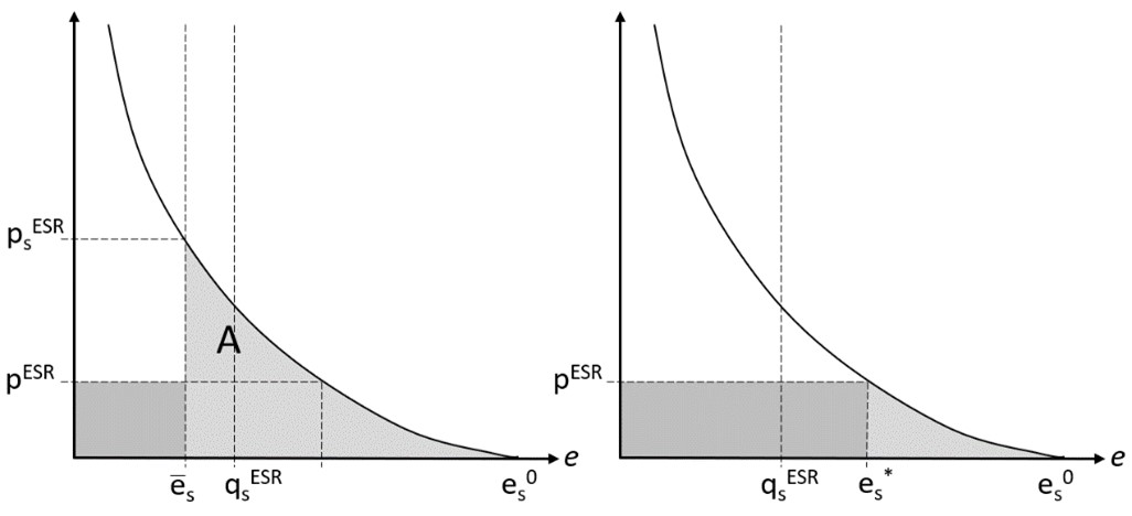
The difference in compliance costs between the two policy strategies equals the avoided costs of domestic abatements (area A) minus the value of the freed-up quota units (v(q_S^{ESR}-e̅_S)). This is the additional cost of a policy that abstains from international emissions trading and aims at a domestic emissions target below the quota allotted by the ESR. It should be noted that this assessment presumes that the country controls its emissions in a cost-effective manner so that abatements are conducted in the order that the MAC curve ranks the options. As previously mentioned, Sweden has a separate emissions target for domestic transport, whereby this requirement is not met.

Figure 3 illustrates how sub-sector targets increase the cost of attaining a given national emissions target. In the figure, the emissions of the transport sector (T) are counted from left to right and the emissions of the residual ESR sector (ESR-T) from right to left. The two subsectors T and ESR-T may together emit e ̅_S (the length of the x-axis). Let q_T denote the sector target for transport and q_{ESRT-T} the target for the ESR-T sector. The allocation q_T,q_{}_{ESR-T} requires that emissions from transport are priced at τ_T while it is sufficient with the price \tau_{ESR-T} in the ESR-T sector. As the figure is drawn, it is possible to reduce the cost of reaching the emission target e ̅_S by letting the transport sector emit more and requiring the ESR-T sector to abate more. The cost-minimising allocation of abatement efforts is given by (e_T^{opt},e_{}_{ESR-T}^{opt}) at which emissions are priced at P_S^{ESR}. Compared to the policy with sub-sector targets, the cost savings correspond to area B.

Figure 3 The additional cost of sub-sector targets

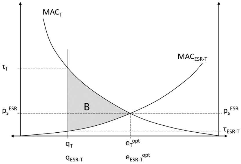
Again, this is an adequate assessment only if the policies within each sector are cost effective. If the policy leads to non-uniform incentives to abate, the control costs will be higher than the figure indicates.

Here, we illustrate how the Swedish climate policy palette creates strong incentives for certain abatement options and low incentives for others, hence reducing emissions in non-cost-effective ways.

The unit cost of reducing carbon-dioxide emissions of fossil origin by means of biofuel standards for diesel and petrol, respectively, can be expressed as

where p_idenotes pump prices and u_fstates the amount of CO₂ emissions from burning a litre of fossil fuel.

The biofuel standard increases production costs with ∆C_R=(1-β ̂ ) p_f+β ̂p_b-p_f=β ̂(p_b-p_f) and reduces the end-of-pipe emissions of fossil origin with ∆e_R=u_f-(1-β ̂〖)u〗_f=β ̂u_f,where \betâdenotes the blending share (in volume terms) that are consistent with β above.

Consider an example for diesel. Assume that p_f=SEK 10 per litre, that p_b=3p_f and that u_f=2.6 kg CO₂. Then, the cost of reducing the CO₂ emissions of fossil origin in the transport sector by blending in biofuel in diesel amounts to SEK 7.7 per kg avoided.

By increasing pump prices, the biofuel standards also have an indirect impact on emissions. The energy and carbon-dioxide taxation increases the diesel price (excl. VAT) with SEK 4.1 per litre (see Table 1). In addition, given a blending share (in volume terms) equal to 0.3, the biofuel standard increases the price of diesel by approximately SEK 6 per litre. The total price increment of this policy combination equals SEK 10 per litre of diesel. Thus, the marginal incentive to reduce emissions by abstaining from buying diesel amounts to SEK 5.5 per kg of fossil CO₂.

SEK 10 per litre divided by (1 - 0.3)2.6  kg CO₂ per litre equals SEK 5.5 per kg.

The results of this example correspond to earlier assessments.

The Swedish Transport Administration (2020a) appreciates the costs of reducing emissions from road traffic by means of electrification or energy efficiency measures to SEK 2–4 per kg CO₂, by blending in biofuels to SEK 1.3–2.6 per kg

The Swedish Transport Administration assumes a smaller price difference between fossil and biogenic diesel as well as a lower price on fossil diesel than in the calculation above.

and through measures reducing traffic to SEK 5.2 per kg. The Swedish National Audit Office (2020) estimates the costs of the bonus allocated to low-emitting cars at SEK 6 per kg CO₂. It should be noted that as a substantial portion of the electricity-fuelled cars sold in Sweden is exported to Norway after a couple of years, the cost increases to SEK 16–19 per kg.

Few instruments target emissions from the ESR sector outside transport. Biofuel mandates and energy and carbon taxation also apply to the use of fossil fuels outside the transport sector. However, the substantial emissions of methane and nitrous oxide are only targeted by small subsidy programmes, which explains the appearance of Figure 1.

The discussion above indicates that the instruments in place for controlling the domestic ESR emissions are leading to an allocation that is potentially far from the cost-effective one.

As mentioned above, the Fit for 55 proposal allocates net-uptake obligations for member states for the period 2026–2030. The finer details are still to be negotiated. However, it seems that Sweden is to be allotted an obligation to accomplish a net uptake in 2030 that is 4 Mt CO₂ higher than the average net uptake during a reference period 2016–2018, which according to the Swedish Environmental Protection Agency (2020) was  43.3 Mt CO₂e. Sweden can achieve this obligation by (i) increasing its storage of carbon in forests and land, (ii) buying LULUCF credits from other countries and/or (iii) using ESR-quota units. All these measures have associated costs.

The net uptake may be increased by reducing the outtake of biomass, employing longer rotation periods, restoring wetlands, reforesting, increasing forest growth by fertilisation and moving the carbon stored in trees to other storage pools (e.g., by constructing durable wooden structures). As mentioned above, Sweden lacks a general policy aimed at controlling carbon storage in its LULUCF sector. Studies therefore indicate that the Swedish net uptake may be increased, at least initially, at rather low costs (NIER, 2021). For instance, Gong and Guo (2017) find that a carbon price/subsidy of SEK 0.17 per kg emission/uptake would increase the storage of carbon in Swedish forests by around 14 million tonnes CO₂. 

At what prices Sweden might buy LULUCF credits from other member states remains unclear. However, the EU Commission (2021) assumes prices at around SEK 0.05 – 0.10 per kg CO₂ uptake in their calculations.

If Sweden does not avail of the options above, then it may have to use ESR-quota units to cover a LULUCF deficit. It can obtain quota units for this purpose in three ways: (i) import of ESR-quota units from other member states at the price P^{ESR}, (ii) annulling fewer ESR-quota units than planned at the unit cost v, and (iii) further reducing its domestic ESR emissions at a unit cost τ_T or \tau_{ESR-T}_{} (in terms of Figure 3). As pointed out previously, with unsuitable instruments, the cost may well be higher.

It should be noted that the EU Commission’s impact assessment of the Fit for 55 calculates a price on ESR-quota units of approximately SEK1.5 per kg carbon dioxide in 2030 (EU Commission, 2020).

This price lies over and above the ‘prices’ implicitly included in the countries’ reference scenarios.

If large high-cost countries abstain from trading, the price could be much lower.

Although annulling fewer ESR-quota units would not implyany financial cost for Sweden, this option would probably carry a political cost, as it would increase the EU’s aggregate emissions.

To further reduce domestic ESR emissions with the sole purpose of fulfilling the LULUCF obligation appears to be the most costly option, given the cost assessment referred to above.  

In all scenarios, the LULUCF regulation implies that there will be a cost associated with using biomass in ways that release carbon dioxide into the atmosphere. Not developing a domestic policy that, to some extent, increases the uptake in the Swedish LULUCF sector may prove sub-optimal in the long term.

The additional costs of the Swedish climate policy, relative to a policy that fulfils Sweden’s EU obligations at the lowest possible cost, consist of the sum of:

In addition, the upcoming LULUCF regulation will introduce a cost for countries using biomass in ways that release carbon dioxide into the atmosphere.

Assessments of the cost savings and other economic consequences of Sweden shifting towards a climate policy that fulfils its EU obligations at the lowest cost possible requires a general equilibrium approach. Such a policy shift would likely produce large changes in domestic energy prices and timber products, giving rise to greater general-equilibrium effects.

Environmental Medium-Term Economic Model (EMEC) is a computable general equilibrium (CGE) model for the Swedish economy. It explicitly captures links between economic activity, energy use and greenhouse-gas emissions and has been tailored to answer research questions about the economic effects of various climate policies. EMEC is formulated as a mixed-complementarity problem using the Mathematical Programming System for General Equilibrium Analysis (Rutherford, 1999). A full description of EMEC is provided in NIER (2023). Here, we restrict ourselves to a description of the basic features of the model and focus on the main climate-policy instruments in place in Sweden, including the EU ETS, domestic energy and carbon taxes and biofuel standards (“Reduktionsplikten”).

Several economic agents interact by demanding and supplying commodities on markets. We specify representative households for six types differentiated by income and residential area. Households enjoy final consumption products and leisure time, own their hours available for work and leisure, have a marginal propensity to save and invest in capital and own the resulting stock of capital.

We specify representative firms across 35 sectors, producing 43 different products in all, where a product can be a good or a delivered service. Production requires capital, labour in the form of working hours and intermediate inputs from other industries, where the inputs can move freely between sectors.

The model includes a government collecting taxes, paying subsidies, consuming final consumption goods and services and paying net transfers back to the households. The government also holds the balance of payment for imports and exports in foreign exchange, and we let the price of foreign exchange adjust endogenously.

The economy is specified as open and small relative to other countries, meaning that world market prices are taken as given. However, domestically produced products are generally assumed to be imperfect substitutes for imported products, allowing for domestic product prices to differ from the world market prices. This is modelled using the formulation in Armington (1969). The markets for labour and capital are assumed to be domestic only.

Agents behave rationally but have imperfect foresight over time.

Households maximise utility (henceforth referred to as welfare) subject to their budget constraint. Welfare is specified as nested-CES

CES stands for constant elasticity of substitution.

functions of leisure hours and bundles of final consumption products, and we measure welfare changes as equivalent variation, i.e., calculating the income change that would give the same welfare change as the policy change. By allowing households to derive welfare from leisure hours, we introduce a trade-off between leisure and consumption and make their supplies of working hours endogenous. Enjoying more leisure hours increases welfare but also decreases labour income, and thus welfare is derived from consumption.

Final consumption products are bundled into multiple consumption bundles. Within the consumption bundle of housing-related products, we distinguish between electricity, district heating and various heating fuels.

As the Swedish transport sector has an individual climate target for 2030 and is subject to substantial policy measures, considerable model development has been conducted regarding this particular sector. Within the consumption bundle of transport products, we distinguish between sea, air, rail, and road transports. Within road transports, we further distinguish between purchased and own road transports. When it comes to own road transports, we further distinguish between own road transports with new and two vintages of used light-duty vehicles. We specify vehicle stocks with the help of capital dynamics equations and with household ownership of these stocks. In addition, the model includes a technology-rich representation of vehicles by distinguishing between multiple types of light-duty vehicles and fuel blends. Specifically, we distinguish between light-duty vehicles with (i) diesel engines running on a diesel blend, (ii) petrol engines running on an E10 blend, (iii) petrol engines running on an E85 blend, (iv) petrol engines running on an E10 blend and electricity (plug-in hybrid electric vehicles) and (v) electric motors. We let the choice of vehicle type for use in own road transports be governed by a CES function over vehicle types and be based on the total user cost of the vehicle and fuels in the current period. We assume a relatively high substitution elasticity for the choice of new vehicle types and a relatively low substitution elasticity for the choice of used vehicle types in own road transports. EMEC is thus able to analyse, e.g., the effects of bonus-malus on emissions through how it affects the vehicle stocks. Similarly, the model can capture how changes in biofuel standards (see below) affect fuel prices and how this, in turn, affects the choices of new vehicle purchases and, therefore, the speed at which electric vehicles are introduced. In this way, the model captures the recent rapid increase of electric vehicles as a share of new cars. We do not specify any scrapping subsidies or exports of used vehicles.

Further, we assume an income elasticity of demand for transport products of less than one to reflect the fact that some household transport demands are non-discretionary (e.g., commuter journeys) and that household transport demands, therefore, increase less than proportional to increases in household income.

Note that environmental quality does not enter the welfare function, implying independence of the demand functions for goods with respect to environmental quality.

Producers maximise profits subject to their production functions, specified as nested-CES functions of capital, working hours, energy, transports and other intermediate inputs.

Within the nest of energy inputs, we distinguish between electricity, district heating and fuels, and we further distinguish between various solid and liquid fuel types (e.g., coal, oil, and gas).

Intermediate use of transport products is specified similarly to the specification of household consumption of transport products. We specify the same choice of light-duty vehicles and fuel blends. In addition, we distinguish road transports between passenger and cargo road transports, further distinguish between purchased and own cargo road transports, and between own cargo road transports with new and two vintages of used heavy-duty vehicles (HDVs). HDVs with diesel engines can run on both the regular diesel blend and a pure biodiesel blend (HVO100). However, we do not specify HDVs with electric engines. We again specify stocks of all vehicles with the help of capital dynamics equations. Since capital is embodied in the vehicles, the households own these vehicle stocks as well.

Constant returns to scale in production and the perfect-competition assumption imply zero profits.

Firms’ production processes, intermediate use of fuel products by firms, and final consumption of fuel products by households give rise to emissions of greenhouse gases and may all be subject to policy and emission prices. Firms subject to the EU ETS need emission permits to emit greenhouse gases. In addition, they may need to pay a domestic carbon tax if the firm, production sector and emission source are subject to the tax. Households may need to pay a domestic carbon tax if the emission source is subject to the tax.

When faced with an emission price, households and firms choose to keep on emitting and pay the emission price, or reduce their emissions and avoid paying the price, or a combination of both, whichever is the cheapest. When choosing to reduce emissions, households have the abatement options of substituting other final consumption products for the polluting one (e.g. choosing less carbon-intensive fuels for own road transports or heating), of substituting low carbon-intensive consumption bundles for high carbon-intensive consumption bundles (e.g. consuming less of the road transport bundle and more of the rail transport bundle), of enjoying more leisure hours instead of consumption bundles, or a combination of multiple abatement options. Similarly, firms have the abatement options of substituting other intermediate inputs for the polluting intermediate input (e.g. choosing less carbon-intensive fuels in own road transports or other parts of their production process), of substituting capital and labour for intermediate inputs (e.g. choosing more fuel-efficient engines in own road transports or other parts of their production process), or by cutting back the production level or a combination of multiple abatement options.

Revenues generated by the auctioning of EU ETS permits flow out of the country (to the EU Commission). The Swedish government does receive a share of total auctioning revenues (from the EU Commission), but this share is exogenous in the model. Domestic carbon tax revenue accrues to the government.

Transport fuel blends are specified as functions of a fuel product and fuel standards. Such a function is specified for each combination of a fuel blend (e.g., E10) and matching fuel products (e.g., petrol and ethanol). Multiple fuel products can thus be sold as the same fuel blend. A set of fuel standards, however, ensures that fuel blends meet minimum and maximum volume requirements on the use of biofuel and fossil-fuel products. For example, we require the E10 blend to have a minimum ethanol volume content of 10% and a minimum petrol volume content of 90% initially.

In the model, the fuel standards are implemented with the help of tradable allowances. This is a way of assuming that fuel distributors can distribute the required emission reductions across fuels in the most economically efficient way. Fuel distributors need to submit certain shares of the biofuel allowance (e.g., 10%) and the fossil-fuel allowance (e.g., 90%) for each litre of the fuel blend. At the same time, fuel blends made from the biofuel product (e.g., ethanol) earn one biofuel allowance per litre sold, whereas fuel blends made from the fossil-fuel product (e.g., petrol) earn one fossil-fuel allowance per litre sold. In case the initial biofuel content is too low, demand for the biofuel allowance will exceed its supply, and the allowance price will increase until it is profitable enough to supply the minimum required amount of the biofuel. The same price setting applies to fossil-fuel permits. We interpret the allowance prices as shadow prices of required cross subsidisation between the fuel products since permits have not been introduced in the real world. These prices change the relative prices of the fuel blends.

In real life, the fuel standard for diesel and petrol, respectively, may trade with each other (i.e., an underachievement in the fuel standard for petrol may be compensated by overachieving for diesel and vice versa). Such trade between fuel standards is not implemented in the current model.

Households and firms solve their respective optimisation problems. Markets for production factors and final goods are assumed to be perfectly competitive. When all markets clear and household income balances hold, the set of output, price and income levels constitute an equilibrium. The equilibrium is static in that the optimisation problems are based on current-period variables only.

We solve for the static equilibrium in the years 2019 through 2050, allowing us to perform a comparative-static analysis of policies in these years. In between these years, we impose several exogenous changes to the model to let the economy grow, as measured in terms of GDP. For example, factor supplies, energy efficiencies and policies can all change. We cannot account for business-cycle behaviour but instead calculate the new equilibria under the assumption that all agents have sufficient time to adjust their behaviour (e.g., choice of the number of hours worked) to the changes imposed.

The model is calibrated to the Swedish economy in 2019. We use the system of National and Environmental Accounts (Statistics Sweden, 2022) as our main data source for economic activity, energy use and emissions of greenhouse gases. World-market prices for fossil fuels (crude oil, coal and natural gas) and EU ETS emission-permit prices are exogenous to the model and are set according to the EU Commission’s recommended parameter values (EU Commission, 2022). Import prices of biofuels (ethanol and biodiesel) are assumed to rise in line with the crude oil price. The base-year calibration reflects a production cost for ethanol that is 1.5 times the cost of petrol per litre, while for biodiesel, the corresponding figure is 2.5 times relative to fossil diesel. Additional model details on transport fuels and vehicles in the base year are calibrated based on several data sources, including the Swedish Energy Agency (2020; 2021) and Transport Analysis (2020). The relative price of electric vehicles has been calibrated with a downward trend over time to reflect exogenous productivity growth and economies of scale, as well as an implicit cross-subsidy from EU regulation on the emission intensity of new vehicles. The model replicates the strong growth in the sales of new electric passenger vehicles in the period 2019 through 2022.

In this section, we assess the additional costs the announced Swedish climate policy imposes on Swedish households relative to a policy that achieves the same greenhouse-gas emission reduction in a more cost-effective manner. We do so by comparing a reference scenario with four policy scenarios. All policy scenarios reach the same greenhouse-gas emissions reduction. In three of them, the entire emission reduction occurs in Sweden. In the fourth, a part of the reduction occurs in other EU member states through trade in ESR-quota units.

The reference scenario is a business-as-usual scenario calibrated to the demographic and macroeconomic development described in NIER (2022) and in which we assume that Sweden’s main trading partners undergo a similar demographic and macroeconomic development. We include only climate and other policies currently in place (up to and including December 2022).

Current policies include the EU ETS, energy and carbon taxes, and biofuel standards (“Reduktionsplikten”) as the primary policy instruments within the Swedish ESR sector. Note that several industry exceptions exist for energy and carbon taxes. Moreover, a carbon tax is also levied on the biofuel products in the E10 and diesel blends covered by the biofuel standards. This means that as long as biofuels are more costly to produce than their fossil counterparts, there are no incentives to raise the biofuel shares in the fuel blends above what is required by the biofuel standards. The E85 and HVO100 blends are assumed to retain the exemptions from carbon and energy taxes that they currently enjoy. In addition, current policies also include an aviation tax, subsidies to certain types of climate innovation

The ‘Klimatklivet’ and ‘Industriklivet’ support schemes.

and ‘bonus-malus’ for new vehicle purchases.

The lump-sum subsidy (the bonus) is reduced to zero from 2023 onwards, while the vehicle tax component (the malus) of the policy is assumed to remain in place.

In the reference scenario, the greenhouse-gas emissions from the Swedish ESR sector fall to a level 51% below the 1990 level by 2030, leaving a gap of 12 percentage points to reach the national target level of 63% below the 1990 level, by 2030. Relative to the 2005 emission level, this represents a reduction of about 48%. In other words, an emissions level close to the Swedish ESR-emission quota suggested in the Fit for 55.

The national target, a 63% reduction relative to 1990, corresponds to a further reduction of about 5 Mt compared to the 50% reduction proposed in Fit for 55. In the four policy scenarios, we specify greenhouse-gas emission reductions equivalent to those implied by this national target, but we do so in different ways (see Table 2).

The first scenario labelled A1, is identical to the reference scenario, but we lift the current set of positive carbon tax rates –with an equal amount– to the levels needed to reach the overall emissions reduction target within the Swedish ESR sector by 2030. That is, we keep the current design of the carbon tax and leave both the carbon tax on the biofuel products in the fuel blends and the industry exceptions in place.

The modelled set of carbon tax levels thus remains differentiated between emission sources and industries.

Note that we do not use any instruments aimed at reducing the emissions of methane and nitrous oxide in the Swedish ESR sector. The reason for this is two-fold. Firstly, such policy instruments would, in the real world, be associated with high transactions costs. Secondly, if implemented unilaterally such a policy would probably jeopardise the Swedish farmers’ competitiveness.

The second scenario, labelled A2, deviates from scenario A1 to reflect current policy proposals. Scenario A2 contains lower biofuel standards for petrol and diesel fuel blends to 15%, which represents our estimate of an EU minimum level in 2030.

In the third scenario, labelled B, we move towards a more uniform carbon taxation. More precisely, we do so by (i) removing the aviation tax, (ii) removing the climate and industry leap subsidies, and (iii) removing the carbon tax from the biofuel components in fuel blends and removing the industry exceptions (other than sea transport) from the tax. As the tax is only levied on the fossil component, it will now influence blend-in levels. However, as the assumption about the EU minimum biofuel standard still applies, the blend-in will never fall below 15%. We again increase the carbon tax to the level needed to reach the emissions reduction targets within the Swedish ESR sector by 2030. It should be noted that the resulting carbon tax is not fully uniform within the Swedish ESR sector due to carbon emissions from sea transports continuing to be exempt from the domestic carbon tax in this scenario and other greenhouse gases being similarly left untaxed.

Note also that the carbon tax within the Swedish ESR sector still differs from the EU ETS price as well as the shadow price of net emissions in the LULUCF sector.

The fourth scenario, labelled C, is identical to scenario B, but with the difference that we now increase the carbon tax exogenously, let the model compute the domestic carbon emission reduction and purchase ESR-quota units from other EU Member States (MS) to make up the difference to the national emission reduction target level of 63% below the 1990 level by 2030. In line with uniform pricing, we set the carbon tax and the quota-unit price at the same level. The quota-unit price is highly uncertain, and we assume a price of SEK 2,000 per tonne CO₂e by 2030. We test the sensitivity of the model results for the ESR-quota price and the LULUCF-certificate price in section 5.6 below.

Table 2 Summary of scenarios

In the four policy scenarios, we keep the saving rates, balance of payments and final consumption by the government fixed at their respective levels, computed in the reference scenario.

The model is not explicitly designed to account for the LULUCF sector. None of the four policy scenarios includes any active measures to increase carbon uptake in Swedish forests. However, the harvesting of forests varies across policy scenarios, mainly due to the variation in carbon tax rates. We control for this effect in the following way. We let the model calculate the amount of carbon stored in either growing forests or in durable timber products. We do this by assuming that the forests grow exogenously, in the same way, across policy scenarios. Using data on carbon uptake in the LULUCF sector from the Swedish Environmental Protection Agency, we calculate net carbon uptake as forest growth (before harvesting) minus total forest harvest plus the share of the harvest that is used in the timber products industry. This measure shows the largest uptake in scenario A2, followed by A1, B and C. We then require purchases of LULUCF credits from other member states in scenarios B and C to cover the difference with respect to the uptake in scenario A1. In scenario A2, the calculated over-achievement in the LULUCF sector allows for the sale of LULUCF credits to other member states. We assume the same price per LULUCF credit as for ESR-quota units, i.e., SEK 2,000 per tonne. The sale or purchase of LULUCF credits does not affect the model results in any material way.

Table 3 summarises the effects of the modelled policies on greenhouse-gas emission levels within the Swedish ESR sector as well as on carbon emission prices and household welfare levels as our main measures of policy cost. Besides studying the costs of the policies in Sections 5.1 through 5.3, we compare the effects on the macroeconomy and transport fuel prices in Sections 5.4 and 5.5 and conduct a sensitivity analysis in Section 5.6.

Table 3 Effects of modelled policies on greenhouse-gas emission levels and CO₂ prices within the Swedish ESR sector and welfare by 2030

Notes: ’trade’ in the scenario name refers to trade in ESR-quota units between EU MS. Carbon prices are in 2019 terms. Welfare is specified as the aggregate welfare of the six household types, and we measure welfare changes as equivalent variation.

In scenarios A1 and A2, the current positive carbon tax rates are shifted upwards with an equal amount to keep the emissions at the target level (reduce the emission by an additional 9% relative to the reference scenario). In scenario A1 in which we keep the biofuel standards at the same levels as in the reference scenario, we find that the maxi­mum tax rate in the set of modelled carbon tax levels increases to SEK 8,300 per/tonne CO₂. This tax level is more than five times higher than the maximum level in the reference scenario and reflects the fact that the Swedish ag­gre­gate marginal abatement-cost function is quite steep. In scenario A2, in which we lower the biofuel standards for petrol and diesel fuel blends to the EU minimum level, we find that the maximum carbon tax level increases to almost SEK 19,000 per/tonne CO₂. Lowering the standards leads to higher carbon emis­sions from the use of the fuel blends and requires higher carbon tax levels to keep the emis­sions at the target level. Given that the carbon tax is also levied on the biofuel component in the fuel blends under the current carbon tax structure, the tax does not provide di­rect incentives to increase the amount of biofuels in the fuel blends. As a result, the current set of carbon taxes must be set at much higher levels to provide in­cen­tives for other abatement options with higher marginal costs to firms and households.

When measured in welfare terms, we find that the additional emission reduction also comes at a cost in both scenarios A1 and A2. The higher carbon tax levels directly increase the cost of production and consumption for many products, de­pend­ing on their carbon intensity. Yet we also find that a part of these cost increases is offset by cost decreases from lower prices of capital, labour and im­port­ed products. Of these three prices, we find that the price of capital falls relatively more due to more carbon-intensive product production also tending to be relatively more capital intensive. Note here that our assumption of free mobility of production factors be­tween pro­duction sectors helps the firms in (especially non-carbon intensive) pro­duction sectors gain from these price decreases. In addition, households respond to the lower wage by working fewer hours and can offset a part of their welfare loss derived from reduced consumption with a welfare gain derived from more leisure hours.

Moving from scenario A1 to A2, we find that the welfare losses are of similar size and that the welfare loss is slightly smaller in scenario A2 than in A1. When decomposing the welfare losses, we find that the lower biofuel standards in scenario A2 worsen the welfare losses of the current non-uniform structure of the carbon tax. Yet, we also find that the lower standards and higher carbon tax levels lead to a higher adoption rate and stock levels of electric vehicles and hence more of the assumed exogenous productivity improvements that come with these. It should also be noted that in scenario A2 a larger share of the regulation rent of the domestic emission target is captured as tax revenues (as opposed to being dissipated in higher production costs for fuels). Since tax revenues are transferred back to the households, this reduces the welfare loss of moving from A1 to A2.

In scenario B, we find that the uniform tax rate needed to keep the Swedish ESR emissions at the target level in 2030 amounts to almost SEK 7,500 per/tonne CO₂. This tax level is again more than five times higher than the maximum tax level in the reference scenario but is lower than the maximum tax level in scenario A1 and much lower than in scenario A2. Given that we now levy the carbon tax more uniformly on more carbon emissions within the Swedish ESR sector and that we now remove the tax from the biofuel components in fuel blends, abatement options with lower marginal abatement costs are incentivised and a lower carbon tax level is sufficient to keep the emissions at the target level in scenario B as opposed to scenarios A1 and A2.

We find that the additional emission reduction comes with a modest welfare loss in this scenario relative to the reference scenario and that the welfare loss is now smaller compared to that in scenarios A1 and A2. In addition to the welfare effects found in scenario A, we now also find a welfare gain due to the removal of the dis­tor­tion costs of the aviation tax, climate and industry leap subsidies and the non-uniform carbon tax structure. That is, cheaper carbon emission abatement options are incentivised elsewhere in the economy and much of the negative income effects attributed to the distortions are reduced or removed in this scenario, compared to the previous scenarios. These cost savings correspond roughly to area B in Figure 3.

In scenario C, we find that the assumed carbon tax and ESR-quota unit price of SEK 2,000 per/tonne CO₂ leads to a greenhouse-gas emission reduction of 36% at home and 27% abroad, compared to the greenhouse-gas emission level within the Swedish ESR sector of 1990, by 2030.

We find that the additional emission reduction now comes with a welfare gain in this scenario relative to the reference scenario and scenarios A1, A2 and B. In addition to the welfare effects found in scenarios A1, A2 and B, we now also find a welfare gain from removing part of the distortion costs of the domestic carbon tax. That is, cheaper greenhouse-gas emission abatement options are incentivised elsewhere in the EU and part of the negative income effect attributed to the domestic carbon tax is here reduced compared to the previous scenarios.

Table 4 shows that the four policy scenarios have different macroeconomic effects as well as different welfare implications.

A contraction of GDP occurs in scenario A1, relative to the reference scenario. As the increasing levels of the set of carbon taxes make production and product prices more expensive, we find that gross production levels decrease. Production levels of goods fall relatively more than those of services, as the production of goods is more carbon intensive than the production of services. Agriculture and forestry are hit particularly hard, followed by transport services and mining and manufacturing. Further, export levels fall slightly more than import levels as import prices become cheaper relative to export prices. Levels of private household consumption decrease in line with higher prices for consumer products and lower household income. Similarly, investments in fixed capital decrease in line with lower household income.

A greater contraction of GDP can be observed in scenario A2, relative to the reference scenario and scenario A1, which is also reflected in gross production levels of goods and services as well as exports and imports. Production in agriculture and forestry again experiences the largest effect, with a fall of over 10% relative to the reference scenario.

These model runs indicate a higher sensitivity of the production in agriculture to the domestic price on carbon than found in some other studies, e.g., Beck et al., (2021). The discrepancy may be explained by differences in how the input factor land is modelled. In the “GreenREFORM” model used in Beck et al., the land area for agricultural production is fixed, whereby a higher carbon price implies lower land rents. In EMEC, on the other hand, land in not explicitly modelled as an input factor. Instead, it is embedded in the factor capital, the price of which does not vary that much in the scenarios. Instead, a higher domestic carbon price lowers the profits in the agricultural sector whereby it shrinks.

Investments in fixed capital fall slightly further relative to scenario A1 and the reference scenario, while household consumption experiences a similar decrease as in scenario A1, relative to the reference scenario.

A lesser contraction of GDP can be seen in scenario B relative to the previous scenarios. We find that the macro-economic effects are qualitatively similar to those in scenarios A1 and A2 but smaller in magnitude, in line with the smaller welfare loss in scenario B. Gross production in mining and manufacturing benefits the least of all the production sectors, as the move to a more uniform carbon tax in scenario B sees its current tax exemption removed.

In scenario C, we see an expansion of GDP relative to the previous scenarios. We find that levels of household consumption and investments in fixed capital increase. In addition, the negative income effect of the carbon tax is reduced, with household income and savings increasing more as a result. Similarly, gross production levels of most goods and services now increase relative to the previous scenarios and the reference scenario. The exception is again mining and manufacturing, where gross production is now lower than in scenarios A1 and B. A sharp fall in the production of biofuels in line with the lower levels for the biofuel standards and carbon tax drives this result in scenario C.

Table 4 Effects of modelled policies on selected macro-economic variables by 2030 (% changes compared to the reference scenario)

Notes: Scenario A1 refers to the current design of the carbon tax and no trade in ESR-quota units with other EU Member States, scenario A2 is identical to A1 but with low biofuel standards for petrol and diesel, scenario B refers to a more uniform carbon tax and no trade in ESR-quota units with other EU Member States and scenario C refers to a more uniform carbon tax and trade in ESR-quota units with other EU Member States. Levels of GDP, gross production, exports, imports, private consumption, and investments in fixed capital are in fixed price terms. Price of capital and labour are in real and 2019 terms.

Table 5 shows the effects of the modelled policy changes on selected transport fuel-blend prices in the four policy scenarios relative to the reference scenario. The prices of the regular petrol and diesel fuel blends change largely in line with the carbon tax level and vary substantially between the policy scenarios. Compared to the reference scenario, we find that these prices are higher in scenarios A1 and A2, that the price increases are less in scenario B and even negative in scenario C.

In absolute terms, the petrol and diesel prices in 2030 in scenario A1 hover around SEK 56 per litre and SEK 57 per litre, respectively. These price levels are of the same magnitude of those found in other studies of this policy scenario, see for instance Swedish Transport Administration (2020b).

The E85 fuel blend, which consists primarily of ethanol, shows smaller price variations across all scenarios. Finally, we find that the prices of HVO100 and electricity mainly follow economic activity and GDP and only exhibit small variations between scenarios. The relatively stable prices of the HVO100 blend and electricity across scenarios means that these fuels gain market shares when the regular petrol and diesel blend experience high price increases, especially in scenarios A1 and A2. This occurs through substitution away from the regular diesel blend and towards the HVO100 blend in HDVs and through faster growth in the share of electric vehicles in new vehicle purchases.

Table 5 Effects of modelled policies on selected transport fuel blend prices by 2030 (% changes compared to the reference scenario)

Notes: Scenario A1 refers to the current design of the carbon tax and no trade in ESR-quota units with other EU Member States, scenario A2 is identical to A1 but with low biofuel standards for petrol and diesel, scenario B refers to a more uniform carbon tax and no trade in ESR-quota units with other EU Member States and scenario C refers to a more uniform carbon tax and trade in ESR-quota units with other EU Member States. Prices of transport fuels are inclusive of all taxes faced by purchasers and are in real and 2019 terms. Prices for the E10 and diesel blends are SEK 28.6 and 29.7 per litre, respectively, in the reference scenario in 2030.

Table 6 reports the sensitivity of our results to key parameter values. We use central parameter values in all sensitivity scenarios except for the parameter subject to analysis. Given the importance of energy use, associated carbon emissions and abatement costs for our findings, we choose the parameters for the substitution elasticities between value added and energy inputs in production, autonomous energy efficiency improvements and the ESR-quota unit price. Further, considering the significance of the prices of fixed capital and imported products in offsetting much of the cost increases associated with the additional carbon emission reduction, we also choose the parameters for the depreciation rate of fixed capital and the (Armington) substitution elasticities between imported and domestic products. We report effects as percentage changes relative to the reference scenario.

The general result from Table 6 is that our findings are robust to the range of parameter values considered. A more uniform carbon tax and allowing for trade in ESR-quota units with other EU Member States in scenario C still provides the best welfare implications for households, followed by a more uniform carbon tax only, in scenario B, and then followed by the current set of carbon taxes presented in scenarios A1 and A2.

Turning to the specific parameters subject to analysis, assuming a higher depreciation rate for fixed capital leads to slightly lower welfare losses in all policy scenarios relative to the reference scenario. A higher depreciation rate for fixed capital decreases the capital stock and increases the price of capital relative to the regular scenarios, all else being equal. Given that capital and energy are net complements in many production sectors, we find that the higher price of capital leads to lower emission levels already in the reference scenario, in turn leaving smaller emission gaps to close in the policy scenarios. As a consequence, we also find that the required carbon tax levels are now slightly lower in scenarios A1, A2 and B relative to the regular scenarios. We find the opposite effects if we assume a lower depreciation rate and report no changes in carbon emission prices for scenario C since these prices are assumed in this scenario.

Assuming higher (Armington) substitution elasticities between imported and domestic products makes the economy more open, decreases the marginal costs to abate carbon emissions and leads to lower emission levels relative to the regular scenarios, all things being equal. As a result, we find that the targeted emission reduction leads to a smaller welfare loss in scenarios A1, A2 and B relative to the reference scenario but also that the welfare gain from international trade in ESR quotas is somewhat smaller in scenario C. We also find that slightly lower carbon tax levels are now needed to incentivise the additional carbon emission reductions in scenarios A1, A2 and B. We find the opposite effects if we assume lower substitution elasticities between imported and domestic products.

Assuming higher substitution elasticities between bundles of capital and labour and bundles of energy products in production leads to slightly lower welfare losses in scenarios A1, A2 and B and a slightly higher welfare gain in scenario C relative to the reference scenario. The higher substitution elasticity increases the opportunities to substitute capital and labour for energy use and lowers the marginal abatement costs, all else being equal. Consequently, slightly lower carbon tax levels are needed to incentivise the additional carbon emission reductions in scenarios A1, A2 and B. We find the opposite effects occur if we decrease the substitution elasticity.

Assuming larger autonomous energy-efficiency improvements in the use of all energy products also leads to slightly lower welfare losses in scenarios A1, A2 and B and a slightly higher welfare gain in scenario C relative to the reference scenario. The reduced energy use results in lower carbon emissions already present in the reference scenario and, in turn, leaves a smaller emission gap to close in scenarios A1, A2, B and C. In scenarios A1 and A2, the smaller emission gap leads to a slightly lower maximum carbon tax level, whereas it leads to a slightly higher carbon tax level in scenario B. The reduced energy use also results in the additional policies leading to a larger emission reduction. Reducing or removing the additional policies then implies that the carbon tax has relatively more carbon emission reductions to incentivise. We find the opposite effects if we assume lower autonomous energy-efficiency improvements.  

Assuming a higher ESR-quota unit price decreases the welfare gains from trade in these certificates in scenario C as additional and more expensive domestic carbon abatement options are now incentivised. We find the opposite effects if we assume a lower quota price and report no changes in results for scenarios A1, A2 and B since no trade is allowed in these scenarios.

Table 6 Piecemeal sensitivity analysis

With the Fit for 55 package, the EU has developed a comprehensive and ambitious climate-policy framework that rests on what essentially are three separate cap-and-trade systems – EU ETS, ESR and LULUCF. In the EU ETS, the trading decisions are delegated to the emitting entities. Their interest in making profits is likely to guide them towards the cost-effective allocation of emission abatements. The ESR and the LULUCF regulations place obligations on the member states’ governments and, to enhance the cost effectiveness of the policy, allow them to trade ESR-quota units and LULUCF credits, respectively. However, the current Swedish climate policy prevents the government from fully engaging in such emissions trading, prescribes larger domestic emission reductions than demanded by the Swedish ESR obligations, implies relatively strong incentives for some adjustments (e.g., switching to biofuels and electricity in transport) and low or no incentives for some other abatement options. As a result, Swedish households incur additional costs.

We have used a computable general equilibrium model of the Swedish economy to assess the economic consequences of various changes in Sweden’s climate policy while keeping the overall climate ambition constant. More precisely, we study the effects of reaching Sweden’s current national emissions targets by (i) reducing the biofuels standard and instead increasing current (positive) tax rates and (ii) reducing the biofuels standard and applying a more uniform domestic carbon taxation regime to reach the same national emission target. We also study the cost savings of a policy reform (iii) that reduces the biofuel standard, implements a carbon-tax regime that provides more accurate incentives for fuel switching (in transport) and avails itself of the flexibility mechanism allowed under the ESR. Here, the domestic carbon tax is set equal to the international price on ESR-quota units (assumed to correspond to SEK 2,000 per/tonne CO₂), and Sweden buys emission-quota units not only to fulfil its ESR obligation but also to attain the same overachievement as planned under the current policy.

The results indicate that a policy that reduces the biofuel standards while raising the current positive carbon tax rates to reach our national emission targets will create high petrol and diesel prices (compare scenarios A1 and A2 in Table 3 and Table 5). To a large extent, such price increments can be avoided by introducing a more accurate and uniform national carbon tax. The benefit of the latter step is equivalent to an income increase of 0.22% in 2030 (compare scenarios A2 and B in Table 3).

However, retaining national emission targets will nonetheless impose additional costs on Swedish households. The model results presented above indicate that abolishing our national emission targets and buying emission-quota units from other member states represents substantial cost savings for Sweden and will not only fulfil our ESR obligation but attain the same overachievement that Sweden’s current policy implies, thereby substituting cheaper abatements in other member states for more expensive ones in Sweden. Given the assumed price on ESR-quota units, the cost savings corresponds to an increase of 1.1% in the Swedish household’s income in 2030 (compare scenario A1 with scenario C in Table 3). The sensitivity analysis conducted indicates that this conclusion is robust. 

These assessments do not capture any adjustment costs of moving from one equilibrium to another and may, therefore, underestimate actual cost savings. Perhaps more importantly, the analysis does not account for the any benefits of Swedish climate policy. The Swedish policy has been motivated by an ambition to generate various demonstration effects, accelerate technological development and facilitate international negotiations. We leave it to the reader to judge if any values foregone by Sweden, by being less of a forerunner, outweigh the quantified increase in Swedish households’ welfare. It should be noted that an EU-wide cost-benefit analysis of the policy reform should also consider the trade gains accruing to the member states that sell emission-quota units to Sweden.

Armington, P. S. (1969). A Theory of Demand for Products Distinguished by Place of Production, International Monetary Fund (Staff Papers), 16(1), 159–178.

Beck, U., Dahl, G., & Kruse-Andersen P. (2021). Carbon Leakage in GreenREFORM – Global climate effects and leakage-adjusted regulation in a national economic model, Danish Research Institute for Economic Analysis and Modelling [DREAM]. Retrieved from https://dreamgruppen.dk/publikationer/2021/maj/carbon-leakage-in-greenreform/

Directive (EU) 2018/2001. (2018). On the promotion of the use of energy from renewable sources. OJ L 328, 21.12.2018, p. 82–209. Retrieved from https://eur-lex.europa.eu/legal-content/EN/TXT/?uri=uriserv:OJ.L_.2018.328.01.0082.01.ENG

EU Commission. (2020). Stepping up Europe’s 2030 climate ambition, Investing in a climate-neutral future for the benefit of our people. Commission Staff Working Document, SWD 2020/176 final. Retrieved from https://eur-lex.europa.eu/legal-content/EN/TXT/?uri=CELEX%3A52020SC0176

EU Commission. (2021).  Proposal for a regulation of the european parliament and of the council amending Regulations (EU) 2018/841 as regards the scope, simplifying the compliance rules, setting out the targets of the Member States for 2030 and committing to the collective achievement of climate neutrality by 2035 in the land use, forestry and agriculture sector, and (EU) 2018/1999 as regards improvement in monitoring, reporting, tracking of progress and review. COM 2021/554 final. https://eur-lex.europa.eu/legal-content/EN/TXT/?uri=CELEX%3A52021PC0554

EU Commission. (2022). Recommended parameters for reporting on GHG projections in 2023. Directorate-General, Climate Action

Gong, P., & Guo, J.  (2017). The potential and costs of increasing forest carbon sequestration in Sweden, Journal of Forest Economics, 29(B), 78–86.

NIER [National Institute of Economic Research] (2019). Transportsektorns klimatmål, Årlig rapport 2019 [Transport sector climate goals]. KI-NR 2019:19 Dnr 2019-401. Retrieved from: https://www.konj.se/publikationer/miljoekonomisk-rapport/miljoekonomisk-rapport/2019-12-11-planerad-politik-nar-inte-transportsektorns-klimatmal.html

NIER [National Institute of Economic Research] (2021). Miljö, ekonomi och politik 2021 – Skogen, klimatet och politiken [The forest, the climate and politics]. KI 2021:30 Dnr: 2021–445. Retrieved from https://www.konj.se/publikationer/miljoekonomisk-rapport/miljoekonomisk-rapport/2021-12-15-svensk-skog-behover-en-starkare-klimatpolitik.html

NIER [National Institute of Economic Research] (2022). Hållbarhetsrapport 2022 för de offentliga finanserna [Public finance’s sustainability report, 2022], KI 2022:2 DNR: 2022-070. Retrieved from https://www.konj.se/publikationer/specialstudier/specialstudier/2022-02-09-langsiktigt-hallbara-offentliga-finanser.html

NIER [National Institute of Economic Research] (2023). EMEC 4 model description [Manuscript in Preparation].

Ovaere, M., & Proost S. (2022). Cost-effective reduction of fossil energy use in the European transport sector: An assessment of the Fit for 55 Package, Energy Policy, 168, 113085

Panorama (n.d.). Panorama visualization tool, A pathway to Sweden's climate goals. https://app.climateview.global/public/board/ec2d0cdf-e70e-43fb-85cb-ed6b31ee1e09

Regulation (EU) 2018/842. (2018). On binding annual greenhouse gas emission reductions by Member States from 2021 to 2030 contributing to climate action to meet commitments under the Paris Agreement and amending Regulation (EU) No 525/2013. OJ L 156, 19.6.2018, p. 26–42. Retrieved from https://eur-lex.europa.eu/legal-content/EN/TXT/?uri=celex%3A32018R0842

Regulation (EU) 2021/1119. (2021) Establishing the framework for achieving climate neutrality and amending Regulations (EC) No 401/2009 and (EU) 2018/1999. OJ L 243, 9.7.2021, p. 1–17. Retrieved from https://eur-lex.europa.eu/legal-content/EN/TXT/?uri=CELEX%3A32021R1119

Rutherford, T. F.  (1999). Applied General Equilibrium Modeling with MPSGE as a GAMS Subsystem: An Overview of the Modeling Framework and Syntax, Computational Economics, 14, 1–46.

Statistics Sweden (2022). National Accounts, quarterly and annual estimates [Data set]. Retrieved from https://www.scb.se/en/finding-statistics/statistics-by-subject-area/national-accounts/national-accounts/national-accounts-quarterly-and-annual-estimates/

Swedish Energy Agency (2020). Drivmedel 2019, Redovisning av rapporterade uppgifter enligt drivmedelslagen, hållbarhetslagen och reduktionsplikten [Reporting on the Fuel act and Sustainability Act], ER 2020:26.

Swedish Energy Agency (2021). Energy in Sweden Facts and Figures 2021 [Data set]. Retrieved from https://www.energimyndigheten.se/4aa0ef/globalassets/statistik/energilaget/energy-in-sweden-2019.xlsx

Swedish Energy Agency (2022). Kontrollstation för reduktionsplikten 2022 [Report on the reduction obligation], Interim report 1 of 2, ER 2022:07. Retrieved from https://energimyndigheten.a-w2m.se/Home.mvc?ResourceId=208637

Swedish Environmental Protection Agency (2020). National Inventory Report Sweden 2020. Greenhouse Gas Emission Inventories 1990–2018. United Nations Climate Change. Retrieved from https://unfccc.int/documents/224123

Swedish Environmental Protection Agency (2022). Naturvårdsverkets underlag till klimatredovisning enligt klimatlagen [Climate reporting under the Climate Act]. NV-08742-21. Retrieved from https://www.naturvardsverket.se/om-oss/regeringsuppdrag/slutredovisade-regeringsuppdrag/klimatredovisning-enligt-klimatlagen-2022/#:~:text=Naturv%C3%A5rdsverket%20har%20redovisat%20underlag%20till,de%20styrmedel%20som%20%C3%A4r%20beslutade

Swedish Environmental Protection Agency (2023a). Nettoutsläpp och nettoupptag av växthusgaser från markanvändning (LULUCF)[Net emissions and removal from LULUCF]. Retrieved from  https://www.naturvardsverket.se/data-och-statistik/klimat/vaxthusgaser-nettoutslapp-och-nettoupptag-fran-markanvandning/

Swedish Environmental Protection Agency (2023b). Utsläpp inom utsläppshandeln och icke-handlande sektorn [Emissions within the emissions trading and non-trading sector]. Retrieved from https://www.naturvardsverket.se/data-och-statistik/klimat/vaxthusgaser-utslapp-i-den-handlande-och-icke-handlande-sektorn/

Swedish Government (2017).  Proposition 2016/17:146. Ett klimatpolitiskt ramverk för Sverige [Climate policy framework for Sweden].

Swedish Government (2020). Proposition 2020/21:180. Promemoria Reduktionsplikt för bensin och diesel – kontrollstation [Reduction obligation for petrol and diesel].

Swedish Government (2022). Proposition 2021/22:243. Pausad höjning av reduktionsplikten för bensin och diesel 2023 [Suspended the reduction obligation for petrol and diesel].

Swedish Ministry of Finance (2022). Beräkningskonventioner 2023 – Metoder för effektberäkningar vid ändrade skatteregler. [Method for tax calculations]. Retrieved from https://www.regeringen.se/rapporter/2022/11/berakningskonventioner-2023/

Swedish National Audit Office (2020). Statliga åtgärder för fler miljöbilar [State measures for more green cars], RiR 2020:1. Retrieved from https://www.riksrevisionen.se/rapporter/granskningsrapporter/2020/statliga-atgarder-for-fler-miljobilar.html

Swedish Transport Administration (2020a). Klimatstyrmedel i infrastrukturplaneringen – en underlagsrapport till infrastrukturplaneringen [Climate control tools in infrastructure planning]. Trafikverkets Publikation 2020:221. Retrieved from http://trafikverket.diva-portal.org/smash/record.jsf?pid=diva2%3A1484834&dswid=1090

Swedish Transport Administration (2020b). Inriktningsunderlag för transportinfrastrukturplaneringen för perioden 2022-2033 och 2022-2037 [Policy documents on transport infrastructure planning] , Trafikverkets publikationer, 2020:186. Retreived from http://trafikverket.diva-portal.org/smash/record.jsf?pid=diva2%3A1484716&dswid=1007

Transport Analysis (2020). Vehicles 2019 [Data set]. Retrieved from https://www.trafa.se/vagtrafik/fordon/