Nordic Economic Policy Review 2025

In this article, we take a Danish perspective to describe wage setting in the public sector in the Nordic countries and explain why wage growth in the public sector is linked to wage growth in the private sector. We provide an empirical analysis of the wage structure in the public sector in Denmark, examine the wage hierarchy between occupations and education groups and compare the findings with the private sector. We also discuss the advantages and disadvantages of the Nordic wage-setting system for the public sector and suggest ways of addressing the challenges faced by the current set-up. 

Keywords: Public sector, wage setting, Denmark

JEL Classification: J24, J31, J45

How should wages in the public sector be determined, and why is it not straightforward? Why do some occupations in the public sector face recruitment problems? These are some of the questions we address in this article based on the work of the Danish Wage Structure Committee.

In 2021, the Danish government decided to set up a committee to conduct empirical analyses of the wage structure in the public sector, investigate the impact of the current wage-setting system and look at options for improvement. The work was concluded in June 2023, and reports summarising the committee’s work are available for download at https://www.loenstrukturkomiteen.dk/afrapportering.

The views expressed in this article are those of the authors and do not necessarily reflect the views of the Committee as a whole.

The public sector is organised differently from the private sector, including the system for wage setting. In this article, we describe the underlying idea behind wage setting in the Nordic countries and discuss the advantages and disadvantages of the current model, e.g. recruitment challenges. Our main focus is on Denmark, but there are many parallels to the other Nordic countries.

The article contains empirical descriptions and analyses of the wage structure in Denmark, with the focus on the wage hierarchy between occupational groups in the public sector. We discuss how to measure wages and why it is difficult to compare wages between occupational groups and across sectors. Both in the public and private sectors, it is difficult to link productivity and wages directly. Output from certain parts of the private production sector, such as a fixed number of corporeal goods, can be quantified and has a market price. However, even in that particular case, the link between individual-level productivity and individual-level wages is noisy. Wages are partly determined by collective bargaining agreements, but imperfect competition in the market can also affect wages, so we expect to see deviations between productivity and wages, especially at the individual level. The issue is further exacerbated in the public sector, where the ‘output’, e.g. care or teaching, is difficult to quantify and price objectively. As a result of these factors, despite careful empirical analysis of the wage structure, we cannot assess whether wages in the public sector reflect productivity or what an objectively fair wage would be.

In the last section of the article, we discuss ways to deal with the shortcomings of the current system. Here, we focus on the recent tripartite agreement that raised wages for certain occupational groups and make suggestions for how the current wage-setting negotiations can be made more flexible.

In this section, we will provide a brief description of the public sector based on some of the Nordic countries and describe wage setting in the public sector in Denmark. For a detailed discussion of differences and similarities in wage setting between the Nordic countries, we refer to Calmfors (2025).

The Nordic countries are characterised by large and generous public sectors responsible for essential welfare services such as health, education, security (e.g., the police force) and for redistributing money across the country and population. Hence, the public sector accounts for almost 30% of total employment in Denmark, Norway and Sweden, significantly higher than the OECD average of around 18% (Lønstrukturkomitéen, 2023e). 

One feature of the public sector is the high proportion of female employees. In Denmark, where the public sector is split into three sub-sectors (municipalities, regions and the state), seven out of ten public employees are women. The proportion of men and women varies across the sub-sectors, mainly because many women are employed in the municipalities and regions (8 out of 10 employees). However, the gender distribution at the state level is about 50/50. There is also a high degree of gender segregation in the public sector. For example, in occupations such as midwifery and nursing, more than 90% are women, while in other occupations, e.g. military staff, under 10% are women (Lønstrukturkomitéen, 2023d). 

The women employed in the municipalities and regions often work in the large health and care sectors or as teachers and childhood educators. The jobs at the state level, e.g. at universities or in the state administration, often require high levels of education, such as long-cycle higher education and are generally less prone to being considered gender stereotypical (Lønstrukturkomitéen, 2023d).

The Nordic countries are small, open economies with high living standards. Both exports and domestic demand (public and private) contribute to economic growth, with trade playing an important role. In these economies, it seems crucial that the wage setting balances competitiveness and real wage growth (see Høgedahl et al., 2024). 

One defining feature is, therefore, the strong tradition of collaboration between trade unions and employers’ associations on the regulation of the labour market. High membership figures for both facilitate collective bargaining processes, which are important to wage negotiations. Traditionally, issues relating to the labour market are negotiated and decided by the unions and employer associations. In addition, tripartite negotiations (“trepartsforhandlinger”) between unions, employers’ associations and the government sometimes target specific issues (such as pensions) or broader issues (like schemes to support businesses during COVID-19). Tripartite negotiations are common in Denmark and Norway but less so in Sweden.

Public-sector wage growth is linked to average wage growth in the private sector. Traditionally, the part of the private sector that is subject to competition from foreign firms has been the first mover in wage negotiations. As a consequence, wage growth in the public sector closely follows wage growth in the part of the private sector exposed to competition from abroad (in Section 4, we explain the Nordic model in more detail).

The principles that underpin wage setting in the public sector date back to the 1950s and are part of the Scandinavian inflation model. In Denmark, the principles were formalised in the 1987 “joint declaration” (fælleserklæringen), which has helped stabilise wages and, therefore, the economy and public finances (Lønstrukturkomitéen, 2023d).

In Denmark, the public sector wage setting is decided during the collective bargaining negotiations in each of the three subdivisions of the public sector (the state, the regions and the municipalities). The negotiations between unions and public employers determine the overall financial framework, and this includes, for example, an agreement about the overall percentage wage increase for all public employees. The financial framework is based on expected wage growth in the private sector. To ensure parallelism in private-sector and public-sector wages, the ‘Regulation Agreement’ (reguleringsordningen) was set up in 1984. It has subsequently been confirmed (with minor variations) in later negotiations and ensures adjustments and restoration of parallelism if wages in one of the three subdivisions deviate from the private sector or expected wage growth deviates from actual wage growth (Høgedahl et al., 2024). The wage trajectory in the private and public sectors has been almost parallel from 1995 to 2021, as illustrated in Figure 2.1, and wage growth in the public sector clearly tracks the private sector very closely. 

Figure 2.1. Hourly wage trajectory for the private and public sector in Denmark, 1995 to 2021.

Note: The hourly wages are not seasonally adjusted. The wage index is set to 100 in Q1 2005.
Source: Based on Figure a, Box 4.2, Lønstrukturkomitéen, 2023d.

The different elements of the public-sector wage-formation processes are essential for maintaining a robust labour market that supports economic stability and public finances. However, the structure also poses some challenges, especially in terms of ensuring adequate adaptation to and responsiveness to economic changes and shocks to the economy. The structure has faced challenges lately, including recruitment problems in certain occupational groups, e.g., nurses in the public sector. In 2021, a major industrial dispute broke out in Denmark when nurses employed by the regions (hospitals) went on strike for more than two months after turning down the agreement negotiated by their union and the regions (the employers). The main point of contention was wages. The dispute ended after a government intervention, as part of which the Wage Structure Committee (Lønstrukturkomitéen) was set up to ensure more knowledge about public sector wages across occupations.

In Section 4, we will discuss the strengths of the public-sector wage-setting model and the challenges it faces.

This section focuses on describing the public-sector wage structure in Denmark. First, we provide an overview and compare average hourly wages across educational and occupational groups. Second, we make a brief comparison of the findings for the public sector with those for the private sector.

The descriptive figures presented in Section 3 are based on reports by the Wage Structure Committee (see Lønstrukturkomitéen, 2023a; 2023b; 2023d). For detailed statistics, we refer to these publications. 

Our description of the wage structure in the public sector focuses on the hourly wage rate. Hourly wages are comparable across full-time and part-time employees, which means that they should reflect a more direct (and comparable) measure of individual productivity than annual earnings. 

Hourly wages can be measured in different ways (standardised measure of hourly wages vs. absence-corrected measure); see Lønstrukturkomitéen (2023g). The perspective we adopt is that of a given employee’s expected pay. Thus, our measure of hourly wages is 2019-values of a standardised measure for hourly wages equivalent to the hourly wage an employee would see in their contract or on their pay slip.

The figures are Statistics Denmark’s ‘standard calculation of hourly earnings’ (standardberegnet timefortjeneste) documented in detail in Statistics Denmark (2024a). The standardised wage measure is unaffected by periods of absence or leave and includes automatic pension contributions whenever they are included as part of the salary/contract (this is standard in the public sector). It does not include pay for overtime. For occupational groups without a maximum number of working hours per year, the working week is set to 37.5 hours. For employees paid according to actual hours worked, absence could affect the standardised hourly wage rate.

This wage measure is not adjusted for sick days, holidays, pay for overtime, etc., but is instead based on all of the hours for which the employee is paid according to their contract, whether the employee was working or absent.

Statistics Denmark’s wage data also contain a measure of the hourly wage rate corrected for absence (sick days, leave periods, holiday, etc.). This measure is referred to as ‘Earnings per hour of performance’ (fortjeneste pr. præsteret time) in Statistics Denmark (2024b) and represents a more accurate measure of the hourly cost to the employer of the employee. It includes the cost (for the employer) of paying the employee when they are absent. In terms of calculating this hourly wage measure, the only difference to the standardised measure of the hourly wage rate is the number of hours included. For the standardised hourly wage rate, all hours the employee could be working (according to the contract) are included, whereas for the corrected hourly wage rate, only the hours in which the employee was actually working are included. As a result, the absence-corrected measure for hourly wages provides a higher hourly wage rate than the standardised measure.

All interpretations and comparisons in the following subsections relate to a society with a large public sector (Denmark). Thus, many of the findings will be similar to what can be observed in other Nordic countries.

Comparing wage rates across occupations or levels of education is complicated. The main complication arises from the fact that wages consist of several components (basic salary, pension contributions, overtime payments, nuisance compensation, etc.), components that do not have equal weighting across different groups. For example, for some education or occupational groups, overtime payments are included in the basic salary, and hours above those specified in the contract are not recorded or compensated separately. For other groups, pension contributions is not part of the wage, and thus, basic salaries might be higher compared to groups with pension contributions as part of their salary package.

Such differences in the composition of the hourly wage rate are illustrated in Figure 3.1 across 50 occupational groups in the public sector.

The 50 occupational groups are defined in detail in the report “Background Report on Other Employment Conditions Set by Collective Bargaining Agreements” (Baggrundsrapport vedr. øvrige overenskomstfastsatte ansættelsesvilkår). Note that the occupational groups are based on occupation and not level of education. Some individuals in particular occupational groups may, therefore, be allocated to different educational groups (Lønstrukturkomitéen, 2023c).

The wages are reported in DKK, and the exchange rate between Euro and DKK in 2019 was 7.47. Figure 3.1 reveals two things. First, when summing up the different wage components, it becomes clear that some of the 50 occupational groups have substantially higher hourly wages than others. The groups with the highest average wage rates are public-sector managers, officers, junior doctors,

Junior doctors may include people with a lot of work experience, as the total group of doctors is only split between ‘senior’ and ‘junior’. In other words, the ‘junior doctors’ category consists of all those not categorised as ‘senior doctors’.

and researchers, and their average hourly wages range from around DKK 340 to 540. The lowest average wage rates, ranging from DKK 165 to 190, are for childcare assistants, cleaning and household assistants, nutrition assistants, childminders and childhood educators, and service assistants. The average wage for doctors is approximately 2.1 times higher than the wages paid to childcare assistants.

The ratio of wages of doctors to childcare workers is of the same magnitude in Sweden and Norway (2.2 in Norway and 2.1 in Sweden).

Most notably, occupations in which individuals have the highest overall levels of education generally have higher combined wage rates. 

Second, the different components of the wage are weighted quite differently across groups. For example, for many of the occupational groups made up of highly educated staff, especially groups characterised by academic-level education, nuisance compensation is a very small share of the total wage. Instead, overtime is embedded in the ‘normal hours’ specified in the contract. However, most of these groups, especially in the public sector, have pension contributions as part of their standard salary package, e.g., psychologists, engineers, and high school teachers. For many of the health or care-related occupations, e.g., social and health care assistants, nurses, and midwives, nuisance compensation constitutes an important part of the total hourly wage rate, despite pension contributions being included in their standard salary packages.

The average wages depicted in Figure 3.1 conceal information about the dispersion within occupation groups.

Examples of dispersion in wages are illustrated in Figure 1.3 in Lønstrukturkomitéen (2023d).

There is a large variation in hourly wages within some groups, e.g. lawyers and economists, whereas wages for teachers, for example, vary far less. Differences in the dispersion of wages between groups stem partly from prioritisation and compromises in wage negotiations between employers and employees in the past, but they also mirror the degree of variation in the type of job and tasks within a certain occupational group. For example, if a group comprises individuals both with and without managerial responsibilities, we expect to see large variation in hourly wages within the group. See also Calmfors (2025) for more detailed information on wage setting and wage negotiations in Denmark (and the other Nordic countries).

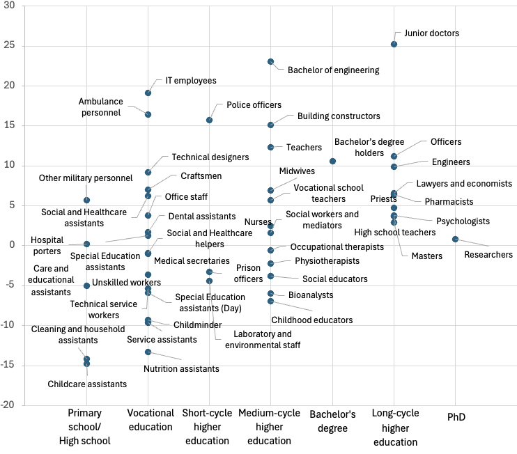
When focusing more specifically on education groups, the relation of higher pay for higher levels of education, suggested by Mincer (1974), is confirmed by Figure 3.1. In Figure 3.2, upper panel, education is divided into eight groups based on individuals’ completed levels of education: primary school, vocational training, short-cycle higher education, medium-cycle higher education, bachelor’s degree, long-cycle higher education, and PhD. The tendency towards a positive association between hourly wages and the length of education is particularly visible in the jump from short- and medium-cycle higher education to long-cycle higher education and PhD. The average wage rate increases by approximately DKK 70 from medium-cycle higher education to long-cycle higher education.

Whenever an education group consists of (many) individuals whose education is a combination of formal and less formal education and training, the registered level for the group can be a bit misleading. For example, the group comprising individuals with short-cycle higher education includes a large proportion of police officers. The basic and mandatory education for police officers is categorised as a short-cycle higher education, but it is common for officers to supplement it with adult and continuing education provided by the Police Academy. This supplemental education is not accredited in the registry used by Statistics Denmark to register the highest completed education, as a result of which police officers are not updated to a higher education group despite relevant supplemental education. In other words, many police officers’ actual levels of education are underreported.

Figure 3.1. The standardised hourly wage rate specified for 50 occupational groups in the public sector in Denmark by wage components.

Source: Based on Figure 1.4, Lønstrukturkomitéen (2023d).

Figure 3.2 The average hourly wage rate in the public sector in Denmark by education group and years of work experience, 2019.

Note: Education groups are based on the highest level of education completed by all public sector employees, excluding students and individuals under 18 years old. Work experience is calculated on the basis of the number of years the employee has paid ATP contributions. Police officers are classified in the short-cycle higher education group, but there is uncertainty regarding their highest completed level of education due to underreporting in the registers of adult and continuing education for police officers.
Source: Based on Figures 3.2 and 3.3, Lønstrukturkomitéen (2023d).

Underreporting has an impact on the overall average hourly wages for the group of short-cycle higher education and implies higher payments for staff with this level of education than would be realistic if police officers were not included. Thus, the wages paid to staff within this education group vary substantially, and there tends to be an upward bias. 

However, even with an upward bias in hourly wages for individuals with a short-cycle higher education, the overall pattern persists of higher wages for higher levels of education. 

When relating hourly wages to work experience, as shown in Figure 3.2, lower panel, an increasing pattern is observed once again. Across all individuals working in the public sector, the longer an individual has participated in the labour market, the higher the average hourly wage rate, at least until about 16 years of work experience. After 16 years, the  returns to work experience on wages becomes almost flat.

The exact point at which the return to work experience flattens out may vary depending on education or occupational groups, but the empirical literature consistently observes this phenomenon over time (see, e.g. Dustmann and Meghir, 2004). The phenomenon is also described as a decreasing marginal return to work experience, implying that those with few years of work experience usually enjoy relatively higher increases in their hourly wages after each year than those with many years on the job. Clearly, that is also the case for workers in the public sector in Denmark.

A simple statistical model in the spirit of Mincer (1974) can be used to further understand the importance of education and work experience as well as other aspects of determinants of the wage rate. Such a model is often used to quantify the association of the actual wage rate with, for example, education and work experience. During the last 20 years, studies have started to look at job tasks as important determinants of wages (see, for example, Autor et al., 2003; and Autor and Handel, 2013). Important job tasks are management tasks, so we specifically include management tasks in our model.

The statistical model used by Lønstrukturkomitéen (2023d) is specified as follows:

An indicator for each level of education is included in the specification, except primary education which is used as the base group, and work experience is included up to cubic terms. An indicator for having management responsibilities is included as well as an indicator for being employed as an (academically trained) manager in the public sector. is the so-called ‘error term’ which includes all factors not observed (or not deliberately included as controls in the model) but which are correlated with hourly wages after taking account of the other variables.

The intuition behind the model can be illustrated as in Figure 3.3, where education, work experience, and management tasks are depicted in green circles as affecting hourly wages directly. Other potentially relevant factors affecting the hourly wage rate are in blue circles. In the statistical model, only education, work experience, and management tasks are quantified directly. The other factors are not included separately, as their impact on wages cannot be objectively measured or categorised through, for example, an economic model as being positively or negatively related to hourly wages. In the following, we will thus mainly consider these (blue) ‘other factors’ as one combined unit. 

Figure 3.3. (Actual) observed wages consist of different components

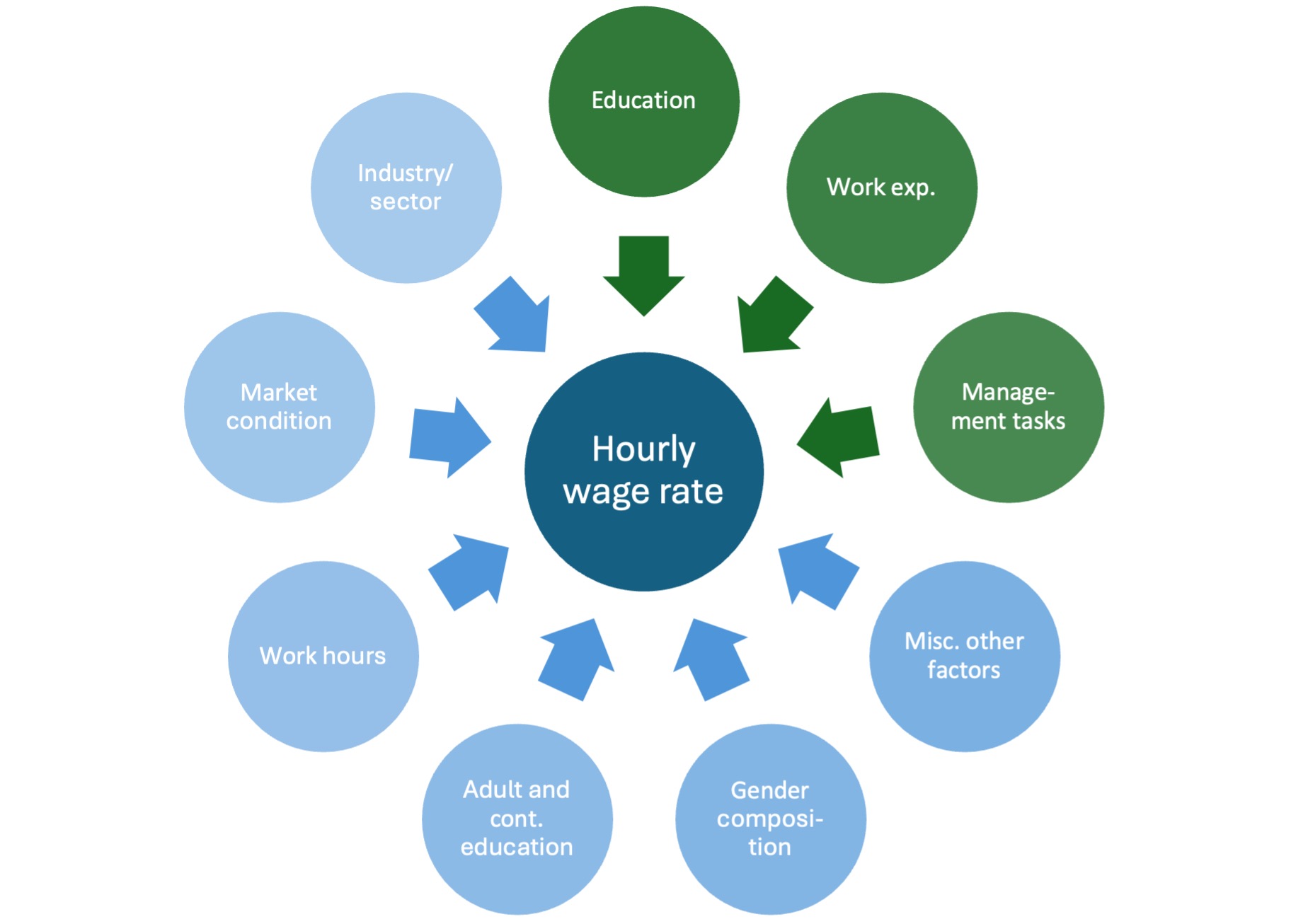
Source: Based on Figure 3.12, Lønstrukturkomitéen (2023d).

When taking only the three green components (education, work experience, and management tasks) into account, the statistical model can explain about half of the variation in the individual wage rates observed in 2019 in the Danish public sector (Lønstrukturkomitéen, 2023d). The implication is that the other half must be explained by other factors, for example, those suggested in the blue circles.

Higher values of the three green components are (on average) positively associated with the hourly wage rate. Based on economic theory (see Mincer, 1974, and Becker, 1964), this positive relation is expected, it is supported by the statistical model, and, as seen in figures 3.1 and 3.2, it also holds true in practice, even when just plotting raw values for education, experience and hourly wages. 

For some occupational groups, factors other than education, work experience, or management tasks might be more (or less) important for the wage rate, for example, some of the factors suggested in the blue circles in Figure 3.3. These other factors could easily move hourly wages in opposite directions and thus, when combined, seem not to be important for determining the wage rate. Therefore, it makes sense to analyse these ‘other factors’ to try to identify potential patterns concealed by the results of the model. For example, if certain occupational groups do a wide range of many different tasks, have different levels of responsibility, or include individuals with systematically different (un)observed characteristics, it will be difficult for the statistical model to accurately predict the actual hourly wage rates.

More formally, when interpreting the outcome of the statistical model, we therefore also investigate how large a part of the observed hourly wage rate cannot be directly associated with education groups, work experience, and management tasks, as this gives us information about the importance of ‘other factors’. For the 50 occupational groups, Figure 3.4 shows how large a portion of the wage rate is not explained by either education, work experience, or management tasks (the unexplained part is formally called ‘the residual’), and it captures the deviation between the actual observed wage rate and the predicted wage rate from the statistical model. The deviations are depicted as a percentage of the average wage rate for each occupational group, and the equivalent value in DKK is specified for a few groups. Deviations between actual and predicted wages for a specific occupational group can be down to either the ‘other factors’ or the fact that the return to wages of education, experience or management tasks for the specific occupation differs from the average.

If the residuals are positive, it means that the sum of the other factors contributes to a higher wage rate for the particular occupation than the statistical model predicts based on education, experience and management tasks. If, on the other hand, the residuals are negative, it implies that, for the particular occupation, the residuals contribute to a lower wage rate. It is important to note that the deviations across all occupational groups sum to zero in total and are thus measured in relation to averages for the whole model and should not be interpreted as absolute values.

It is also important to note that predicted wages do not (necessarily) reflect productivity and, importantly, that predicted wages cannot be interpreted as ‘fair’ or correct wages. The predicted wages solely describe the average  return of education, experience and management tasks for the occupation and how these factors are rewarded under collective agreements.

The statistical analysis shows major deviations between predicted and actual hourly wages for the occupational groups that have the lowest absolute wages on average. Particularly for occupations such as cleaning assistants or different types of childcare or elderly care assistant jobs, the observed average hourly wages are lower than the model predicts. An important reason for the model overshooting the expected hourly wage is that little or no education or training is required to fulfil the formal qualifications for these occupations. As such, some people in these occupations have more education and training than formally required, for example, if they have taken a formal education and later changed their career path. In such cases, the statistical model includes the (high) educational inputs from the completed formal education and predicts that they are not paid according to their educational qualifications. However, in practice, they might be paid according to their qualifications and productivity in terms of the actual tasks they perform, and the statistical model does not account for that when it only includes a measure of the highest completed level of education.

The occupational groups for which the statistical model more often predicts that individuals are paid more than their educational qualifications, work experience and management tasks suggest include engineers, doctors, teachers, and police officers. For some of these groups, there could be hidden (from the model) qualifications, e.g. when supplemental education or training is not registered as an increase in the highest completed level of education. Thus, the wages for a given education group could be artificially high, as is the case with police officers, for example. However, having a higher actual wage rate than statistically predicted could also be a sign of particularly demanding or dangerous tasks or ones requiring a high level of responsibility. The statistical model does not observe such job characteristics, and they would, therefore, be categorised as unexplained reasons for higher (or lower) observed wages. However, the observed differences could also merely be driven by unpaid overtime, which is not captured by the standardised hourly wage rate.

Figure 3.4. Deviations in actual hourly wages and predicted hourly wages by occupational groups in Denmark, 2019.

Note: Deviations between actual wage and predicted wage as a percentage of the predicted wage.
Source: Based on Figure 3.7, Lønstrukturkomitéen (2023d).

It is also important to note that what is presented here are the average wages for each of the occupational groups. Within each group, there is also variation in how precisely the statistical model predicts actual wage rates. This implies that a worker in an occupational group with a relatively low average wage can be paid more than a person from an occupational group with a relatively high wage. Hence, there is a lot of overlap in the wage distribution between occupational groups (further illustrated in Figure 3.9 by Lønstrukturkomitéen, 2023d).

If we shift the focus to education groups, as in Figure 3.5, and zoom in on the most typical education group for each occupational group, we can group occupations by their most typical education group. This exercise leads to the emergence of interesting patterns: within each education group, there is a lot of variation in the size of the unexplained part (the residuals) from the statistical model’s hourly wage predictions despite the model being based on education, work experience, and management tasks. The observed differences in the accuracy of predicted wage rates for the same education group but across occupations are a clear sign of occupational differences in the tasks and roles assigned to people within the same education group. For example, focusing on medium-cycle longer education, midwives have a higher actual wage rate than the statistical model predicts, whereas physiotherapists have a slightly lower actual wage rate than the model predicted.

As illustrated in subsection 3.1, comparing wage rates across occupational groups in the public sector can be complicated. However, it becomes even more challenging to compare wages across sectors. There are several reasons for this, which are also described in detail by Lønstrukturkomitéen (2023).

Within occupational groups, tasks are not necessarily the same across sectors, and it can be difficult to define occupational groups in similar ways across sectors. The payment scheme varies a bit across sectors, e.g. due to differences in pay during lunch breaks, pay for extra working time, and different priorities (or timing) in collective bargaining negotiations between employers and employees’ organisations. Also, since wages in the public sector do not necessarily reflect a balance between demand and supply of labour but are instead partly driven by political decisions, wages in the private sector adjust differently to over- or under-supply of labour. This latter issue is discussed further in Section 4.

A final complication is related to the fact that some jobs might only exist, or to a limited extent exist, in one of the sectors, e.g. police officers, priests, and military personnel in the public sector, and bus drivers and check-out assistants in the private sector. A meaningful comparison across sectors is thus limited to some occupational groups.

With these caveats in mind, we will attempt to compare hourly wages in the public and private sectors. When comparing hourly wages across the whole public and private sectors, as shown in Figure 3.6, one perhaps surprising result is that median hourly wages are almost identical. However, the average hourly wages are not the same across sectors. The average hourly wage in the private sector is slightly higher than in the public sector, DKK 279 vs. 257, but the variation in hourly wages is greater in the private sector. Thus, those with the lowest hourly wages have a relatively lower hourly wage in the private sector than in the public sector, but those with the highest hourly wages in the private sector have a relatively higher hourly wage than those with high hourly wages in the public sector. In short, hourly wages tend to be less compressed in the private sector than in the public sector.

Figure 3.5. Deviations in actual hourly wages and predicted hourly wages by occupational groups and typical education groups, Denmark, 2019.

Note: Occupations are grouped by their most typical education group.
Source: Based on Figure a, Box 3.3, Lønstrukturkomitéen (2023d).

Figure 3.6. Wage distributions in the public and private sectors in Denmark, 2019.

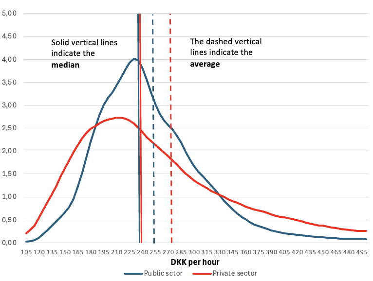
Source: Based on Figure 1.6, Lønstrukturkomitéen, 2023d.

When comparing hourly wages across sectors but within occupational groups as opposed to overall comparisons across the sectors, the average hourly wages are generally similar within occupations across sectors.

We also find that impact of education is similar across sectors, see Figure 67 in Lønstrukturkomitéen (2023a).

The differences between sectors seem to stem from differences in hourly wages among academic groups.

At the same time, when focusing on each education group separately, we also observe some differences in median hourly wages across sectors when not categorising by occupational groups (see Figure 4a in Lønstrukturkomitéen, 2023). Thus, depending on the level and type of subgroup analysis, we do find some differences both in median and average hourly wages across the public and private sectors, and one general result is that hourly wages are higher in the private sector, but the distribution of wages is less compressed in the private sector than the public sector.

In this section, we describe the strengths of and challenges facing the wage setting model for the public sector in the Nordic countries (see also Lønstrukturkomitéen 2023e, 2023f). We start by formally describing the link between wages in the public and private sectors before focusing on the implications of this link for the wage structure and then looking at recruitment issues in the public sector. We again focus on the Danish case to exemplify the particular strengths of the model and the challenges it faces.

As explained in Section 2, overall wage growth in the public sector follows the pattern for wage growth in the private sector, which is mainly driven by the part of the private sector facing competition from abroad. This is a key feature of the wage setting system in the Nordic countries. In the following, we explain the theoretical reasoning behind linking wage growth in the public sector to wage growth in the private sector. 

The premise underlying Nordic wage setting is that the countries are small, open economies and that a large proportion of the firms in the private sector face competition from abroad. In Denmark, about half of the jobs in the private sector were affected by exports in 2011 (Copenhagen Economics, 2018). In the private sector, labour and capital are important inputs into production and hence directly affect firm costs through wages to the workers and cost of capital. In an open economy, where foreign firms can sell products on the domestic market and domestic firms can export, certain industries face (more) competition from abroad. For the firms mostly affected by foreign competition, it is difficult to raise product prices. Thus, high labour costs will cut their profits and can lead to lower production and employment. Therefore, in a market economy with perfect competition, wages should reflect the value of labour and wage growth should be partly determined by productivity and product prices. The theoretical implication is that, in the long run, real wage growth is determined by growth in productivity. However, in the short run, there can be deviations due to business cycles, unemployment, demand and supply of labour and products. Negotiations between unions and employers’ associations are crucial for determining wages and wage growth in the private sector in the short run, see Calmfors (2025).

The public sector is fundamentally different from the private sector because it is not structured as a private market. The demand for publicly provided services is politically determined, and the services are rarely priced in a market. It is, therefore, extremely difficult to measure public sector productivity. This implies that the aggregate wage growth cannot be linked to growth in productivity and changes in the prices of the services. Instead, wage growth is linked to wage growth in the private sector, particularly the part of the private sector subject to competition from abroad. The theoretical reason for this link is that the two sectors compete to attract labour from the same pool. If wage growth in the public sector exceeds wage growth in the private sector, workers would (to a larger degree) prefer public employment as the wages are higher. Private firms would then have to raise wages, introduce less labour-intensive production, or cut production, all of which will lead to higher firm costs.

In this framework, the strengths of the Nordic wage setting model are fourfold. First, it protects the competitiveness of domestic firms and thus indirectly promotes exports. Second, the model contributes to stable prices and ensures that real wages follow the pattern for productivity growth in the long run. Third, it ensures stable public finances. Fourth, it provides a stable balance between the private and public sectors, facilitating recruitment in both. However, it does not rule out recruitment issues in specific areas.

This framework can explain the general idea behind the wage setting model, but it is far too simple to provide a description of all aspects of public wage setting. The model does not take account of the fact that there are different types of labour and that different subsectors may require a certain type of labour (either in terms of education or experience). In addition, productivity growth may vary between subsectors and industries. Whereas productivity is quantifiable in the private sector to a great extent, and local wage setting can account for differences in productivity or excess demand for certain types of labour, it is less straightforward in the public sector.

One of the consequences of the public-sector wage setting model in Denmark has been that wage growth for different occupations has been almost the same. Although nothing in the system imposes similar wage growth for all occupations, this is historically what has happened. One possible explanation is that an overall framework for collective bargaining sets an overall reference point for wage growth in the public sector. If one occupational group has higher wage growth, other groups have lower wage growth than the reference point, and, in this perspective, the negotiations in the public sector can be viewed as a zero-sum game. Over the years, attempts have been made to make wage setting more flexible. In the 1990s, “new pay” (ny løn) was introduced, emphasising that part of the wage negotiations should be conducted locally in public-sector workplaces. At present, 8–10% of total wage growth is negotiated locally, a proportion that has only increased slightly in the last 15 years.

To investigate whether wages in the public sector react to market forces, for example, to excess demand in certain occupations, we plot deviations between actual and predicted wages against the rate of unsuccessful recruitment.

The rate of unsuccessful recruitment is based on a survey of firms by STAR. The occupational groups in the survey and in the register data do not correspond exactly, so we have matched the occupational groups. For some groups we do not have a measure of unsuccessful recruitment due to too few replies being received.

The scatter plot in Figure 4.1 shows no evidence of a correlation between the ‘residuals’ and unsuccessful recruitment (the correlation is less than 0.05). This indicates that the wage process in the public sector does not adjust to excess labour demand and that the public sector is likely to face recruitment challenges. 

We also investigate whether wages in the public sector adjust to competition for labour from the private sector. We define occupations in which a large proportion of the staff works in the private sector as ones that face competition over labour because the employees could probably find alternative employment in the private sector. The analyses confirm that occupations in which more than 80% work in the private sector (e.g. engineers, IT employees and craftspeople) have higher wages in general (when accounting for education, experience and management tasks). However, there are also exceptions. It is possible to find occupations where, for example, unskilled workers receive a relatively low wage in the public sector, despite 70% of people in the occupation working in the private sector, see Lønstrukturkomitéen (2023b). This suggests that wages in the public sector only partly adjust to competition for labour with the private sector.

Figure 4.1. Scatter plot between deviations of actual and predicted hourly wages and unsuccessful recruitment.

Source: The deviations between actual and predicted wages are based on Figure 3.7, Lønstrukturkomitéen (2023d). The measure of unsuccessful recruitment rate is based on surveys by STAR (see https://jobindsats.dk/databank/arbejdsmarked/status-pa-arbejdsmarkedet/virksomhedernes-behov-for-arbejdskraft/virksomhedernes-forgaeves-rekrutteringer/). The correlation between deviations and unsuccessful recruitment rate is 0.049.

When the relative wage growth across all occupations in the public sector is almost similar, one consequence is that relative wages do not adjust over time to productivity changes or excess demand for certain types of labour. This implies that if productivity in certain occupations increases, then the wages in the private sector will probably go up, but this will not necessarily be reflected in public-sector wages. Hence, wage growth in certain subgroups may not be parallel in the public and private sectors despite parallel aggregated wages in the two sectors. The empirical analyses in Lønstrukturkomitéen (2023) provide some support for this observation. For example, doctors in the private sector have an hourly wage of around DKK 500, while doctors in the public sector earn around DKK 350 per hour.

Lately, discussions in Denmark have often centred around the wage structure being rigid and thus, to some extent, reflecting the wage structure many years ago. A comparison of the wages paid to different occupational groups in the public sector in 2010 and 2019 confirms that the wage hierarchy has remained almost unchanged over the decade (see Lønstrukturkomitéen, 2023g). In this light, debate has raged about whether occupations traditionally dominated by women have a lower wage because the wage structure in the public sector has remained almost unchanged. Lønkommissionen (2010) found that the main driver of the gender wage gap was wage differences between occupations rather than wage differences between men and women in the same occupation. Women are more likely to be employed in occupations with lower wages, and thus, when taking into account occupation, experience and education, the gender wage gap is only 0.5–3% (Lønkommissionen, 2010).

Similar evidence is found in the work by Lønstrukturkomitéen (2023), in which the focus was on wages in the public sector. Analyses indicate that female-dominated occupations in the public sector have lower wages even when education and experience are taken into account. As an example, IT employees (less than 20% of them are women) have substantially higher wages than nutrition assistants (more than 80% women), even though both groups have a vocational education. In fact, nutrition assistant wages are only 70% of an IT employee’s pay.

When wages in the public sector cannot adjust to productivity changes and recruitment challenges, the public sector comes under pressure in both the short run and the long run. The demographic trends towards an ageing society will increase the demand for labour in the care sector. To illustrate the problem, the Ministry of Finance has presented analyses of recruitment issues for specific occupations in Denmark, for example, nurses and teachers (Finansministeriet, 2022). These empirical analyses look at both excess demand in the short run (2022) and predictions for excess demand in 2030 (given rather strict assumptions).

To empirically quantify the excess demand for certain types of labour in the short run, the Ministry of Finance analyses the number of vacant positions or positions that are filled with individuals without the requisite skills/competencies. These analyses point to an excess demand for nurses and staff in the elderly-care sector and show that the excess demand has risen from 2019 to 2021. Another aspect of excess demand is regional differences. In the capital region, the number of vacancies is high for nurses but low for doctors, whereas in other regions, there are more vacant positions for doctors than for nurses. 

A different way of analysing recruitment is by investigating the proportion of employees who leave a given occupation for another one or leave the labour market entirely. The empirical analyses suggest that childhood educators and social and health assistants, in particular, leave the public sector. In the period from 2014 to 2019, 37% of childhood educators and social and health assistants left the public sector.

These two different recruitment analyses indicate that there is excess demand for nurses, childhood educators and social and health assistants in Denmark at the moment (2022). The Ministry of Finance also analyses the excess demand for labour in 2030 for the same subset of occupations. In this exercise, a number of assumptions are made, leading to an almost mechanical prediction based on 1) a forecast of the expected number of new graduates with certain qualifications (given the current graduation pattern), 2) the number of employees expected to leave the job; and 3) the future demand for labour based on demographic trends. The Ministry of Finance estimates that in 2030 there will be substantial excess demand, especially for social and health assistants. The mechanical predictions suggest excess demand of around 17,000 people. However, these calculations do not account for adjustments in the labour market. 

In a market economy, we expect imbalances or excess demand to disappear in the long run as the labour market adjusts. First of all, wages are an important adjustment mechanism. If wages for one occupation go up, the job becomes more attractive. This probably implies that more part-time workers will increase their working hours and that people with relevant education and skills in other jobs will return to their occupations. In the long run, we would also expect higher wages to result in more applicants for education for the occupation concerned as the education becomes relatively more attractive because of the high wages (or low unemployment rate). A second adjustment mechanism is the substitution of types of labour. If there is excess demand for a certain type of labour, other occupational groups can take over certain tasks. We already see this happening, for example, in hospitals, where tasks previously done by nurses are now done by other groups. However, this kind of transfer of responsibility for tasks is not always simple, as it could lead to demands for higher wages from the group taking over the responsibility. Third, automation or other technological innovations may affect the demand for labour in the future (and have already done so in the past). Fourth, targeted immigration can also change the supply of labour for certain occupations, for example, attempts to hire nurses from abroad in order to fill vacant positions in hospitals. Fifth, a somewhat different adjustment mechanism is related to outsourcing work; that is, work previously done in the public sector can be done outside of the public sector (but could still be paid for by the public sector).

The analyses presented by the Ministry of Finance assume that none of these adjustment mechanisms are present, which means that there is a risk of overestimating the excess demand. It is a political decision which adjustment channels to use, but they are means to deal with excess demand of labour in the long run, and the choice of mechanism will probably also depend on the severity and expected duration of the recruitment problem.

The Nordic wage setting model has many strengths. First, the fact that the public sector cannot have permanently higher wage growth than the private sector protects the competitiveness of firms and indirectly supports exports. Second, the model contributes to stable prices, wages and public finances, and third, it provides a balance between the private and public sectors, such that the public sector is always able to recruit staff.

The main challenges are related to the fact that the wage setting does not respond perfectly to (excess) supply and demand within and between occupations. Thus, although aggregated wage growth in the public sector follows growth in the private sector, these trends are not necessarily parallel at the occupation level. This can lead to problems retaining and recruiting employees in certain occupations. At the same time, it is difficult to accurately predict future excess demand or excess supply of labour in different occupations. Predictions are currently based on certain (mechanical) assumptions and thus cannot take natural or politically regulated adjustments in the labour market into account.

The model has some built-in rigidity, which has sparked debates about the need for adjustments in relative wages, particularly from groups in the public sector who feel under-compensated compared to their private-sector counterparts or whose occupations are paid less than other occupations with similar levels of education and training.

In the introduction, we posed questions such as ‘How should wages be determined in the public sector? Why is it difficult to set wages in the public sector? Why do some occupations face recruitment problems?’ In later sections, we described some of the challenges in determining wages in the public sector as well as how and why some occupations face recruitment problems. We will now discuss suggestions for addressing the challenges faced by the current wage setting system, for example, suggestions for principles for reforming and developing the current system within the overall framework of the Nordic wage setting system. We will also discuss a recent tripartite agreement between unions, public employers and the government on wages in the public sector in Denmark.

One of the main problems with the current system is the fact that wage growth is often the same for all occupational groups, and wages do not always reflect excess supply or excess demand. This has sparked a discussion of how to change the system for wage setting in the public sector to make it more flexible and able to adjust to a greater extent to imbalances such as excess demand for labour. The Danish Wage Structure Committee formulated four overarching principles for public-sector wage setting (Lønstrukturkomitéen, 2023d). These principles can be used as a starting point for a discussion of how to reform the current system under the premise that wages are set jointly by the unions and employers’ associations and that the overall trend for public-sector wages should be parallel with the private sector.

The four principles are:

Whereas “Transparency” and “Proportionality and legitimacy” are designed to ensure that wage setting is considered legitimate, the last two principles aim to make it more flexible and able to address issues such as excess demand for labour and recruitment challenges. In particular, “Adaptability” has been introduced to make wages in the public sector more adaptable to labour demand and supply shocks and to prevent recruitment problems. “Supportive of task completion” suggests that wage setting can reward certain tasks that are crucial for public-sector delivery. When drawing up the four principles, the Committee also came up with 15 specific suggestions for wage setting (Lønstrukturkomiteen, 2023d).

See Section 8, “Idékatalog for udvikling af løndannelsen i den offentlige sektor” in Lønstrukturkomitéen (2023d).

These suggestions are examples of ways to fine-tune the system within the framework of the Nordic model. The suggestions address issues such as adjustments between and within occupational groups, but not all of the suggestions are equally attractive to the organisations representing both employers and employees.

Once the Wage Structure Committee had completed its work, the Danish government initiated tripartite negotiations concerning wages and the working environment in the public sector between the government, unions and the public employers. The negotiations were to focus on sectors and occupational groups currently (2023) facing recruitment problems. In December 2023, the government, unions and public employers reached an agreement, which involved wage increases, primarily for social and health assistants, childhood educators, nurses and prison officers.

Trepartsaftalen om løn og arbejdsvilkår, 4. december 2023 (Trepartsaftalen, 2023).

The agreement ensured an extraordinary rise of DKK 6.8 billion annually to the budget for public employees.

The annual budget increase for the public sector was DKK 3 billion (after tax, etc.).

The point of the extraordinary increase was to increase labour supply, especially in the health and elderly care sector and, in particular, to ensure a high enough supply of employees willing to work evening, night and weekend shifts. To achieve this, salary supplements were introduced. For example, the agreement contains a wage supplement after four years of tenure as a social and health assistant in the health or elderly care sector. This supplement can be seen as a way of retaining employees in the sector. Specific wage increases for staff working evening, night and weekend shifts have also been introduced as well as means of retaining older employees by improving the scheme for employees above the age of 58. The tripartite agreement also contains permanent wage increments for specific occupations such as social and health assistants, childhood educators, childcare assistants and prison officers, groups that had relatively low wages compared to others (see Figure 3.5). However, the tripartite agreement also contains elements to ensure greater flexibility by employees, e.g. by increasing the maximum number of working hours to 12 per day. As part of the agreement, public employers are also committed to initiating a discussion about adapting the wage setting system to make it more flexible. 

The tripartite agreement was an extraordinary event, and it is explicitly stated in it that this type of agreement will not be repeated. It deviates from the normal procedure in two ways. First, this wage negotiation was not part of the ordinary wage negotiation and involved the government (which normally does not take part in collective bargaining). Second, the wage budget was increased by DKK 6.8 billion (above what would be implied by the growth in the private sector).

The recent tripartite agreement in Denmark addresses some current and urgent recruitment problems and imbalances in the public sector. However, it does not in itself prevent other imbalances in the future caused by changes in the demand for public services or changes in the labour supply. Adapting the Nordic wage setting model for the public sector so that it is always able to cope with such changes remains a challenge.

Given that the wage setting models in the Nordic countries have many similarities, especially because all of them have large public sectors, national experiences provide valuable input into adjustments to the procedure. Sharing experiences on how to gather relevant information on wages and on successful adjustments to economic shocks or imbalances can help shape discussions about the future of the Nordic wage setting model for the public sector.

Autor, D. H. & Handel, M. J. (2013). Putting tasks to the test: Human capital, job tasks, and wages. Journal of Labor Economics, 31, 59-96.

Autor, D. H, Levy, F., & Murnane, R. (2003). The skill content of recent technological change: An empirical exploration. The Quarterly Journal of Economics, 118, 1279–1333.

Becker, G. S. (1964). Human Capital. New York: National Bureau of Economic Research.

Calmfors, L. (2025). Pattern bargaining as a means to coordinate wages in the Nordic countries. Nordic Economic Policy Review. https://pub.norden.org/nord2025-001/pattern-bargaining-as-a-means-to-coordinate-wages-in-the-nordic-countries.html

Copenhagen Economics (2018). Betydning af international handel for økonomi og beskæftigelse i Danmark.Erhvervsstyrelsen. Retrieved from copenhageneconomics.com/wp-content/uploads/2021/12/copenhagen-economics-2018-betydning-af-international-handel-for-oekonomi-og-beskaeftigelse-i-danmark.pdf

Dustmann, C., & Meghir, C. (2005). Wages, experience, and seniority. The Review of Economic Studies, 72, 77-108.

Finansministeriet (2022). Rekrutteringsforhold i den offentlige sektor.

Høgedahl, L., Ibsen, C. L., & Ibsen, F. (2024). Public sector wage bargaining and the balanced growth model: Denmark and Sweden compared. European Journal of Industrial Relations, 30, 55-75. Retrieved from https://doi.org/10.1177/09596801231188511

Lønkomissionen (2010). Faktaark: Lønkommissionen.

Lønstrukturkomitéen (2023). Baggrundsrapport vedr. sammenligning af timeløn for offentlige og private grupper. Retrieved from www.loenstrukturkomiteen.dk/media/kuybvjox/baggrundsrapport-vedr-sammenligning-af-timeloen-for-offentlige-og-private-grupper.pdf

Lønstrukturkomitéen (2023a). Baggrundsrapport vedr. statistiske analyser af lønstrukturer i den offentlige sektor (Trin 1). Retrieved from www.loenstrukturkomiteen.dk/media/e4xare2d/baggrundsrapport-vedr-statistike-analyser-af-loenstrukturer-i-den-offentlige-sektor-trin-1.pdf

Lønstrukturkomitéen (2023b). Baggrundsrapport vedr. supplerende analyser af lønstrukturer i den offentlige sektor (Trin 2). Retrieved from www.loenstrukturkomiteen.dk/media/ynmhn4mu/baggrundsrapport-vedr-supplerende-analyser-af-loenstrukturer-i-den-offentlige-sektor-trin-2.pdf

Lønstrukturkomitéen (2023c). Baggrundsrapport vedr. øvrige overenskomstfastsatte ansættelsesvilkår. Retrieved from www.loenstrukturkomiteen.dk/media/q5tedbx1/baggrundsrapport-vedr-teknisk-afgraensning-af-offentlige-personalegrupper.pdf

Lønstrukturkomitéen (2023d). Lønstrukturkomitéens hovedrapport. Retrieved from www.loenstrukturkomiteen.dk/media/m3klvrmg/loenstrukturkomite-ns-hovedrapport.pdf

Lønstrukturkomitéen (2023e). Baggrundsrapport vedr. Nordiske erfaringer og perspektiver på offentlig løndannelse. Retrieved from www.loenstrukturkomiteen.dk/media/byxbay0x/baggrundsrapport-vedr-nordiske-erfaringer-og-perspektiver-paa-offentlige-loendannelse.pdf

Lønstrukturkomitéen (2023f). Baggrundsrapport vedr. effekter og konsekvenser af ændrede lønstrukturer i den offentlige sektor. Retrieved from www.loenstrukturkomiteen.dk/media/h35hgza5/baggrundsrapport-vedr-effekter-og-konsekvenser-af-aendrede-loenstrukturer-i-den-offentlige-sektor.pdf

Lønstrukturkomitéen (2023g). Baggrundsrapport vedr. beskrivelse af lønstrukturer i den offentlige sektor. Retrieved from www.loenstrukturkomiteen.dk/media/ixvlheqy/baggrundsrapport-vedr-beskrivelse-af-de-offentlige-loenstrukturer.pdf

Mincer, J. (1974). Schooling, Experience, and Earnings. New York: NBER Press.

Statistics Denmark (2024a). Documentation of the standardized wage measure. Retrieved from www.dst.dk/da/Statistik/dokumentation/Times/loenstatistik/fortj-stand

Statistics Denmark (2024b). Documentation of the absence-corrected wage measure. Retrieved from www.dst.dk/da/Statistik/dokumentation/Times/loenstatistik/fortj-prae

Trepartsaftalen (2023). Trepartsaftalen om løn og arbejdsvilkår, 4. december 2023. The Ministry of Employment. Retrieved from: bm.dk/media/rotljv5b/trepartsaftale-om-loen-og-arbejdsvilkaar.pdf
bm.dk/media/quhc5txu/trepartsaftale-om-ekstraordinaert-loenloeft-til-faengselsbetjente-vaerkmestre-og-transportbetjente-i-kriminalforsorgen.pdf