Nordic Economic Policy Review 2024

This paper discusses recent research on the distribution of income and wealth as determinants of fiscal multipliers and the implications for economic policy in the Nordic countries. Economies with higher wealth inequality or lower income inequality have been shown to have more low-wealth and credit-constrained consumers. These consumers have less of an elastic labour supply response to fiscal policies that change their future income but more of an elastic response to policies that change their current income. The labour supply elasticity across the wealth distribution drives the fiscal multiplier. Nordic countries are characterised by high wealth inequality and low income inequality, two features associated with a large number of credit-constrained and low-wealth households. Thus, we expect fiscal stimulus programmes that increase consumers’ current income to have more of an impact in the Nordic Region and programmes that increase future income to have less of an impact.

Keywords: fiscal multipliers; wealth inequality; income inequality, asymmetry

JEL Classification: E21, E62, H31, H50

We would like to thank the editors, Jouko Vilmunen and Juha-Pekka Junttila, our discussant Tord Krogh and participants at the NEPR conference in Reykjavik in November 2023 for their helpful comments and suggestions. Holter is grateful for support from the Research Council of Norway, grant numbers: 302661 (IMWEL), 219616, 267428 (OFS), and 341250 (NFS). Holter also thanks the Portuguese Science and Technology Foundation (FCT), CEECIND/01695/2018, PTDC/EGE-ECO/7620/2020, 2022.07354.PTDC, UIDB/00124/2020 and Social Sciences DataLab, PINFRA/22209/2016). Ferreira thanks the Portuguese Science and Technology Foundation (FCT), SFRH/BD/144996/2019.

Like other OECD countries, the Nordic nations use fiscal stabilisation policies to cushion the impact of business cycles and unforeseen events, such as the recent COVID-19 crisis. In response to the 2008 financial crisis, many countries pursued expansionary fiscal policies (see Figure 1), often financed by debt. Government deficits exceeded 10% in many of them, and this created an urgency for fiscal consolidation policies as soon as times returned to normal. Different policymakers and researchers appear to have had quite different expectations regarding the impact of the fiscal policies pursued, and the ensuing academic literature has actually broadened our views in this regard. As a result, the idea has emerged that there is no such thing as a fiscal multiplier. Instead, the multiplier now appears to be viewed as a function of national characteristics, the state of the economy, the type of fiscal instrument deployed and the size of the fiscal stimulus; e.g., Ilzetzki, Mendoza, and Vegh (2013), Brinca et al. (2016), Brinca et al. (2021), Brinca et al. (2023).

Figure 1. Government Spending as Percent of GD

Source: OECD (2023)

In this paper, we review some of the recent research on the determinants of fiscal multipliers and discuss the findings in light of the characteristics of the Nordic economies. Based on the results in Brinca et al. (2021), we also provide estimates of fiscal multipliers for the Nordic countries in the context of fiscal consolidation. Brinca et al. (2016) found that countries with greater wealth inequality have larger fiscal multipliers when they finance higher government spending by means of current lumpsum taxes. Brinca et al. (2021) showed that the fiscal multipliers resulting from fiscal consolidation programmes in Europe after the financial crisis were larger in countries with higher income inequality. Brinca et al. (2023) found that fiscal multipliers are increasing in the spending shock, with more expansionary government spending shocks generating larger multipliers and more contractionary shocks generating smaller multipliers.

All three of the recent research papers by Brinca et al. (2016), Brinca et al. (2021) and Brinca et al. (2023) have emphasised the importance of low-wealth and credit-constrained households for fiscal multipliers. In all three papers, the mechanism works through the proportion of such households in the economy. As is well known in the economic literature, the elasticity of intertemporal substitution (EIS) is increasing in wealth

See Domeij and Floden (2006) for the relationship between wealth and the EIS of labour and Vissing-Jørgensen (2002) for the relationship between wealth and the EIS of consumption.

, with constrained agents having the lowest EIS. Thus, the labour-supply elasticity of constrained and low-wealth agents in response to contemporaneous changes in income is higher. On the other hand, the hours worked by constrained and low-wealth agents are less responsive to future income shocks. Brinca et al. (2016) focus on a fiscal experiment in which higher government spending today is financed by a lumpsum tax, i.e., changes in transfers to households are used to finance the change in government spending. Under this fiscal policy, the labour supply of low-wealth consumers is highly elastic, and the fiscal multiplier proves to be more substantial in economies characterised by a higher prevalence of credit-constrained consumers. Letting heterogeneous discount factors be the source of wealth inequality and calibrating their model to match cross-country wealth distribution, the authors find that countries with greater wealth inequality have more credit-constrained households and, thus, larger fiscal multipliers.

In Brinca et al. (2021), the focus is on fiscal consolidation after the financial crisis. Various countries drew up plans to reduce debt over several years through austerity measures, tax hikes or a combination of the two. In this paper, the authors first show empirically that there is a positive correlation between higher income inequality and the size of fiscal multipliers induced by fiscal consolidation episodes. They then build a macro model with heterogeneous agents and incomplete markets to explain this observation. Also here, the mechanism works through the labour supply elasticity across the wealth distribution. In economies with more income risk, there is more precautionary saving and, thus fewer agents located close to the borrowing constraint. Fiscal consolidation programmes have a negative effect on output today through a future income effect. As government debt is paid down, the capital stock and thus the marginal product of labour (wage rate) rises, and thus expected lifetime income increases. As a result, agents enjoy more leisure and cut their labour supply now, and output falls in the short term, despite the positive long-term effects of consolidation on output. Credit-constrained agents and agents with low wealth do, however, have a lower marginal propensity to consume goods and leisure out of future income. Economies with higher income risk have fewer credit-constrained consumers, and as a result, the effects of fiscal consolidation programmes are greater.

Finally, Brinca et al. (2023) argue that the fiscal multiplier is increasing in the spending shock, with more expansionary government spending shocks leading to larger multipliers and more contractionary shocks to smaller ones. They document that empirically, this holds true across time, countries and types of shocks. The mechanism again hinges on the elasticity of labour supply across the wealth distribution as well as a shift of the wealth distribution in response to shocks.

Nordic countries are characterised by a combination of high wealth inequality and low income inequality (both pre-tax and post-tax), which suggests there are large numbers of borrowing-constrained and low-wealth consumers in the Nordic economies. These are individuals or households who may have limited access to credit and financial resources and are more likely to increase their spending when they receive additional income from government programmes today. This, in turn, magnifies the fiscal multiplier effect of programmes that have an impact on income today (for example, the Bush tax credits

All taxpayers received a check in the mail.

), as these consumers have a higher propensity to consume goods and leisure from contemporary income. At the same time, the fiscal multipliers from programmes that affect consumers’ future income are reduced. We would, therefore, expect the fiscal multiplier from programmes providing direct transfers to households to be large in the Nordic countries. On the other hand, fiscal consolidation programmes that involve reducing government spending or increasing taxes to reduce government debt over time tend to affect consumers’ future income, and we expect the fiscal multipliers from such programmes to be relatively small in the Nordic Region. In Section 4, we present different estimates of multipliers from fiscal consolidation programmes in OECD countries, in which the Nordic average ranges from 0.98–1.47 compared to an average of 1.20–1.77 for all of the countries in the sample.

The remainder of the paper is structured as follows. In Section 2, we present some stylised facts for the Nordic countries. We look at their fiscal systems as well as the distributions of earnings and wealth. In Section 3, we review recent research on the impact of the earnings and wealth distributions on fiscal multipliers and on the sensitivity of fiscal multipliers to the size of the fiscal shock. Section 4 discusses the implications of this research for the Nordic countries. We present our conclusions in Section 5.

Before diving into an analysis of fiscal multipliers in the Nordic countries, we will describe some features of their economies. In particular, we will look at their income and wealth distributions, but also their use of fiscal stabilisation policies and, to complete the picture, certain features of the Nordic welfare states which may have contributed to shape the income and wealth distributions.

Nordic economic policies are characterised by a combination of free market activity and government intervention, leading to the creation of a welfare state. All the countries that belong to the Nordic Council have targets or limits for fiscal balance and are committed to counter-cyclical fiscal policies (Gylfason et al., 2010). In some cases, it may be useful to distinguish the ones that belong to the European Union (EU) – Denmark, Finland and Sweden – and the ones that do not – Iceland and Norway – as the EU has its own guidelines for fiscal policy. The Nordic countries are known for their welfare states, consisting of various transfer and social insurance programmes. The Nordic welfare states were built up gradually in the years after World War II when the countries introduced high, progressive tax rates to finance welfare services.

For EU member states, the Union’s fiscal rules include a ceiling for the nominal fiscal deficit of 3% of GDP, a structural balance and an expenditure benchmark requiring that higher government spending is matched by additional discretionary revenue measures. Denmark and Finland have incorporated these rules into their national policies, but Sweden has not. In 2000, Sweden introduced a new fiscal rule with a target of a government surplus of 1% of GDP on average over the business cycle. Iceland and Norway, which are outside the EU, set their own fiscal objectives. Iceland’s target is that total liabilities must be under 30% of GDP. For Norway, the fiscal target is a structural budget balance for the central government after withdrawals from the oil fund. The structural non-oil deficit is allowed to vary over the business cycle and should, over time, be equal to the expected real return of the oil fund (Gylfason et al., 2010).

In the early 1990s, Sweden, Finland and Norway introduced the Nordic Dual Income Tax (DIT) system, which combines a flat tax on capital income with a progressive labour tax. Notably, labour taxes in the Nordic countries exhibit a higher degree of progressivity, especially compared to the United States but also to the European average, as shown in Table 1. Due to the implementation of the dual-income tax system, the Nordic countries tend to have very high and progressive tax rates on labour income in international comparisons but somewhat lower flat tax rates on capital income.

The Nordic countries are strongly committed to reducing income inequality by setting progressive tax rates that impose heavier burdens on higher earners. All the countries have a property tax and a value-added tax. The latter is quite high by international standards. In addition, Norway applies a tax on net wealth. Denmark abolished this tax in 1997, Sweden in 2007. In all of the countries, property tax is seen as a way to tax wealth. However, as this tax is levied on every household that owns its own home, it does not distinguish households with mortgages from those where the property is exclusively an asset. This means that it does not consider net household wealth.

Compared with other economies, the Nordic countries have high tax-to-GDP ratios, meaning that in these countries, a relatively large fraction of production goes to the government budget (see Table 2) and can be spent on health, education and other redistributive measures. These values have been relatively stable over time in the Nordic countries.

Table 1. Tax measures by country

Source: Average consumption, labour and capital tax are retrieved from Trabandt and Uhlig (2011). No data is available for Norway and Iceland. Income progressivity tax index data is retrieved from Holter et al. (2019).

 

Table 2. Total tax burden by country (2020)

Source: OECD (2022)

As mentioned previously, the Nordic countries have a distinctive economic profile characterised by a notably low level of income inequality (see Table 3 for income inequality measures by country). The countries also have relatively high wealth Gini coefficients by international standards, indicating significant wealth disparities. As we will discuss below, this intriguing duality in income and wealth dynamics assumes paramount significance when considering the impact of fiscal policy on the nations’ economies.

The low income Gini coefficients underscore that policies directed at income redistribution, such as progressive taxation and robust social welfare programmes, may be having the desired effect. The economic literature shows that progressive tax and transfer policies may even affect pre-tax income inequality in addition to their direct redistributive effect. However, other factors, such as strong trade unions, may also influence the pre-tax income Gini coefficients. An interesting point is that none of the Nordic countries have a statutory national minimum wage. Wages are negotiated by trade unions and the employers’ organisations. Conversely, we observe that the wealth Gini coefficients are high in the Nordic countries. Fully understanding the drivers of wealth and income inequality is beyond the scope of this paper, but perhaps the fact that Nordic countries have relatively low flat tax rates on capital income and high and progressive tax rates on labour income is a reason why wealth inequality is particularly high. Another contributor may be the generous social security systems, which reduce the incentive for individuals to save, see Kaymak and Poschke (2016).

Table 3 provides data on the Gini coefficients for income and wealth in North America and Europe. The Nordic countries all have levels of income inequality well below the sample average. The average Gini coefficient for income is 0.32, for example, compared to 0.26 in Norway, 0.27 in Sweden and Iceland, 0.28 in Finland and 0.29 in Denmark.

Turning to the wealth Gini, the Nordic countries appear much more unequal. The differences between them are also greater, with Finland having one of the lower Ginis in the sample and Denmark having the highest. The average Gini coefficient for wealth is 0.67, compared to 0.61 in Finland, 0.63 in Norway, 0.66 in Iceland, 0.74 in Sweden and 0.81 in Denmark. This underscores the fact that, while income inequality is relatively low in the Nordic countries, wealth inequality remains comparatively higher. Both characteristics suggest the presence of numerous low-wealth and credit-constrained individuals, perhaps somewhat dependent on the underlying drivers of the distributions. Brinca et al. (2016) found that economies with more unequal wealth distribution had more credit-constrained individuals. In that paper taxes, social security and heterogeneous discount factors were allowed to vary between countries and shape the wealth distribution. Brinca et al. (2021) shows that income inequality caused by idiosyncratic income risk leads to more precautionary savings and fewer households close to the borrowing constraint.

Table 3. Income and wealth inequality by country

Note: Gini coefficients for wealth are taken from Davies et al. (2007), and Gini coefficients for income are from Brinca et al. (2020). The retrieved values correspond to the year 2000.

The effects of different types of fiscal policy in different states of the world have been a topic of special interest to researchers and policy makers. The literature now seems to agree that there is no such thing as a fiscal multiplier but that the effects of fiscal policy depend on the fiscal instrument, the state of the economy and perhaps also the size of the fiscal stimulus, see among others Heathcote (2005), Auerbach and Gorodnichenko (2011), Ilzetzki, Mendoza, and Vegh (2013), Krueger, Mitman and Perri (2016), Brinca et al. (2016), Brinca et al. (2021), Ferriere and Navarro (2020), Brinca et al. (2023). In this section, we review some of the recent literature on the determinants of fiscal multipliers. We focus on three papers: Brinca et al. (2016), Brinca et al. (2021) and Brinca et al. (2023), and finish up with a brief summary of other related research.

The fiscal multiplier is the change in output resulting from a change in government expenditure. Often one is interested in the impact multiplier:

where is the change in output from period 0 to period 1 and is the change in government spending from period 0 to period 1. The cumulative multiplier at time T can be defined as:

,

where is the change in output from period 0 to period t and is the change in government expenditure from period 0 to period t. There is considerable variation in the estimates of fiscal multipliers across time, location and the method used to finance fiscal policies. Blanchard and Leigh (2013), for example, find that the International Monetary Fund’s (IMF) average forecast of the fiscal multiplier prior to the fiscal consolidation programmes introduced after the 2008 financial crisis was about 0.5. They do, however, show that the IMF systematically underestimated the fiscal multiplier.

Brinca et al. (2016) study the impact of wealth inequality on the effectiveness of fiscal policy. They reveal that countries with greater wealth inequality tend to have more pronounced economic responses to increases in government spending. The starting point is an empirical analysis similar to the one performed by Ilzetzki et al. (2013) to identify the impact of different factors on fiscal multipliers across countries and time. Brinca et al. (2016) use their data and methods to study the impact of wealth inequality on fiscal multipliers. The metric for wealth inequality is the Gini coefficient, taken from Davies, Sandstrom, Shorrocks and Wolf (2007). The authors split the sample into two groups—countries with Gini coefficients above and below the sample mean—and run structural vector autoregressions (SVARs) for the two groups separately. They find that the group of countries with above-average Ginis have a significantly higher (and thus, by assumption, common) fiscal multiplier. Countries with greater wealth inequality have a statistically significant and positive response to an increase in government consumption up to almost two years after the shock, while the group of low-inequality countries does not exhibit this pattern. This can be seen in Figure 2, where a 1% increase in government consumption has a stronger effect on output in countries that have a wealth Gini coefficient above the average (left panel) than countries with one below it.

Figure 2. Fiscal multiplier by wealth inequality

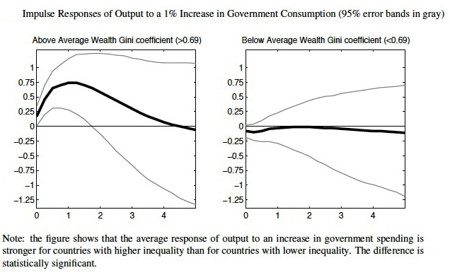
Note: Impulse responses of output to 1% increase in government consumption.
Source: Brinca et al., 2016

Motivated by this stylised fact, Brinca et al. (2016) then develop a model based on modern, quantitative macroeconomic theory with heterogeneous consumers to ask whether differences in the distribution of wealth across countries can lead to differences in their respective aggregate responses to fiscal policy. They focus on a classic fiscal-policy scenario: a one-period unexpected increase in government expenditures financed by a one-period increase in lumpsum taxation (see, e.g., Baxter and King (1993)). Their model is a life-cycle, overlapping-generations (OLG) economy with uninsurable labour market risk, i.e., a life-cycle extension of Aiyagari (1994). The authors calibrate the model to match data from a number of OECD countries along the relevant dimensions such as the distribution of income and wealth, taxes, social security and the level of government debt.

Brinca et al. (2016) find that the size of the fiscal multiplier is highly sensitive to the fraction of liquidity-constrained individuals in the economy. Importantly, it also depends on the average level of wealth. Agents who are liquidity-constrained have a higher marginal propensity to consume goods and leisure, and they respond more strongly to fiscal shocks that change their current income. Larger labour-supply responses, in particular, lead to larger output responses. The marginal propensity to consume is also higher for relatively wealth-poor agents since they have a precautionary savings motive. Finally, relatively wealth-poor economies have a higher real interest rate, and the net present value of an otherwise equally large fiscal shock today is larger when the interest rate is higher. We should, therefore, expect fiscal multipliers to be high in countries with high inequality, a low savings rate and/or a high debt.

In a multi-country exercise, in which they calibrate the model to country-specific data from 15 OECD countries, the authors find that countries with greater wealth inequality have more credit-constrained and low-wealth consumers and, therefore, larger fiscal multipliers. They obtain raw correlations between the fiscal multipliers generated by their model and the wealth Ginis and capital-output ratios of 0.62 and -0.68, respectively. The regression coefficients when the fiscal multiplier is regressed on the Gini or on K/Y are, moreover, highly statistically significant. They find that an increase of one standard deviation in the wealth Gini coefficient for the countries in their sample raises the multiplier by about 17% of the average multiplier value. This finding leads to an expectation of higher multipliers in countries with high wealth inequality – as is the case of the Nordic countries.

Brinca et al. (2021) study the fiscal multipliers resulting from empirically plausible fiscal policies that have been at the centre of the recent policy debate, namely the debt consolidation events that took place after the 2008 financial crisis. They argue that the recessive impacts of fiscal consolidation programmes are stronger when income inequality is greater. They begin by documenting a strong positive empirical relationship between greater income inequality and the fiscal multipliers resulting from fiscal consolidation programmes across time and place. They use data and methods from two recent, state-of-the-art empirical papers: i) Blanchard and Leigh (2013) and ii) Alesina et al. (2015).

They then study the effects of fiscal consolidation programmes financed through both austerity and taxation in a neoclassical macro model with heterogeneous agents and incomplete insurance markets. They show that such a model is well-suited to explain the relationship between income inequality and the recessive effects of fiscal consolidation programmes. The mechanism works through idiosyncratic income risk. In economies with lower income risk, there are more credit constrained households and households with low wealth levels due to less precautionary saving. Importantly, these credit-constrained households have less elastic labour supply responses to increases in taxes and decreases in government expenditure.

The first empirical exercise is a replication of the recent studies by Blanchard and Leigh (2013) and Blanchard and Leigh (2014), which find that the International Monetary Fund underestimated the impacts of fiscal consolidation in European countries. Brinca et al. (2021) reproduce the exercise conducted by Blanchard and Leigh (2013), now augmented with different metrics for income inequality. They find that during the consolidation in Europe in 2010 and 2011, the forecast errors are larger for countries with greater income inequality, implying that inequality amplified the recessive impacts of fiscal consolidation. For example, a one standard deviation increase in income inequality, measured as Y10/Y90,

The ratio of the top 10% income share over the bottom 10% income share.

leads the IMF to underestimate the fiscal multiplier in a country by 66%.

In the second independent analysis, Brinca et al. (2021) use the Alesina et al. (2015) fiscal consolidation dataset from 12 European countries covering the period 2007–2013. Alesina et al. (2015) expand the exogenous fiscal consolidation dataset, known as IMF shocks, from Devries et al. (2011), who use Romer and Romer’s (2010) narrative approach to identify exogenous shifts in fiscal policy. Again, Brinca et al. (2021) document the same strong amplifying effect of income inequality on the recessive impacts of fiscal consolidation. A one standard deviation increase in inequality, measured as Y25/Y75, increases the fiscal multiplier by 240%.

To explain these empirical findings, the authors develop an overlapping generations economy with heterogeneous agents, exogenous credit constraints and uninsurable idiosyncratic risk. They calibrate the model to match the data from a number of European countries along dimensions such as the distribution of income and wealth, taxes, social security and debt level. Then, they study how these economies respond to a gradual reduction in government debt, either by cutting government spending or increasing labour income taxes.

When debt is reduced by cutting government spending, households will shift their savings to physical capital, leading to an increase in the future marginal product of labour and, consequently, in future wages. This positive lifetime income shock leads to a decrease in labour supply and output in the short run. However, in the long run, the economy will converge to a point with more capital and higher output. Credit-constrained agents and agents with low wealth do, however, have a lower marginal propensity to consume goods and leisure out of future income (for constrained agents, the marginal propensity to consume out of future income is zero). Constrained agents have a lower intertemporal elasticity of substitution and do not consider changes to their lifetime budget, but only changes to their budget in the current period.

When fiscal consolidation involves raising taxes on labour income, it has a dual impact on labour supply. On the one hand, there is an income effect that can be positive or negative, depending on whether higher taxes or higher future wages dominate. For constrained agents, the income effects are positive because they do not take the future wage increase into consideration. On the other hand, the tax also induces a negative substitution effect from lower current net wages, which leads to a drop in labour supply. Unconstrained individuals prefer to decrease their labour supply today and utilise their savings or even borrow to maintain a consistent level of consumption. However, constrained individuals do not have the luxury of smoothing consumption in that way. They are compelled to increase their labour supply to avoid a significant drop in consumption. The drop in labour supply will thus be smaller for constrained agents or can even be positive if the income effect dominates.

When higher income inequality reflects more uninsurable income risk, there is a negative relationship between income inequality and the number of credit-constrained agents. Greater risk leads to more precautionary saving, which decreases the share of agents with binding liquidity constraints and low wealth. Since unconstrained agents have a higher intertemporal elasticity of substitution of labour and, thus, more elastic labour-supply responses to both tax-based and austerity-based consolidation, labour supply and output will respond more strongly in economies with higher inequality. This creates a correlation between fiscal multipliers and income inequality.

Brinca et al. (2021) conduct a cross-country analysis for 13 OECD countries in which they calibrate their model to match a wide range of different country characteristics, where, in addition to the distribution of income and wealth, they match data on taxes, social security and government debt. They show that even when introducing substantial country heterogeneity, they are able to reproduce the cross-country relationship between both tax-based and spending-based fiscal consolidation and income inequality.

Figure 3. Impact multiplier and variance of log wages

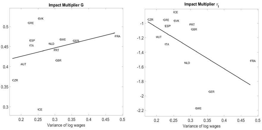
Note: Impact multiplier and variance of log wages. On the left, the cross-country data for a consolidation implemented by decreasing government expenditure, and on the right the cross-country data for a consolidation implemented by increasing the labour tax. Source: Brinca et al. (2021).

Although the mechanism in Brinca et al. (2016) and Brinca et al. (2021) is ultimately the same, it is relevant to highlight that low income inequality does not imply low wealth inequality, as can be seen in Table 3. In fact, Brinca et al. find close to zero cross-country correlation between wealth and income inequality. An important message from these two papers is that both wealth and income inequality can be determinants of the transmission of fiscal policies.

More recently, Brinca et al. (2023) introduced the concept of nonlinear fiscal multipliers. Most of the literature on fiscal policy treats the fiscal multiplier as one number: small and large shocks are assumed to have the same relative effects. Brinca et al. (2023) argue that fiscal multipliers from government spending shocks are increasing in the shock. In other words, large negative shocks yield smaller multipliers, while large positive shocks yield larger multipliers. They first present empirical evidence of this pattern and then show that it can be generated by a standard calibrated neoclassical model with incomplete markets and heterogeneous agents. The key mechanism, which hinges on the differential response of labour supply across the wealth distribution, is robust to assumptions about the form of financing and survives the introduction of nominal rigidities in the context of a Heterogeneous Agents New Keynesian (HANK) model. This type of model serves as a standard framework for examining fluctuations in aggregate demand in the literature.

The authors empirically motivate their paper by borrowing data and methodology from two well-known empirical studies (Alesina et al. (2015)

The same data set as in Brinca et al (2021).

and Ramey and Zubairy (2018)). They find evidence of the size dependence of fiscal multipliers across time periods, countries and types of shocks. In their first empirical exercise, they adapt the methodology and data from Alesina et al. (2015), who use annual data on exogenous fiscal consolidation shocks identified via a narrative approach in 15 OECD countries during the period 1981–2014. They find the multiplier to be significantly — both quantitatively and statistically — larger for smaller fiscal consolidation shocks, with the effect being stronger for unanticipated rather than for anticipated shocks. They also find the results to be similar in the event of both spending-based and tax-based consolidations.

In the second empirical exercise, Brinca et al. (2023) borrow the data and methodology from Ramey and Zubairy (2018), who use quarterly data for the US economy going back to 1889 and an identification scheme for government spending shocks that combines news about forthcoming variations in military spending and the identification assumptions of Blanchard and Perotti (2002). Using the projection method in Jorda (2005), the authors find evidence that the fiscal multiplier increases with the size of the shock. This confirms the finding that the multipliers of larger consolidations are smaller than those of smaller negative fiscal shocks.

A standard neoclassical macro model with incomplete markets and heterogeneous agents can account for these empirical findings. The model is calibrated to match key features of the US economy, such as the income and wealth distributions, hours worked and taxes. The equilibrium features a positive mass of agents who are borrowing-constrained. As discussed previously, the elasticity of intertemporal substitution (EIS) is increasing in wealth, with constrained agents having the lowest EIS. Thus, the labour supply elasticity of constrained and low-wealth agents is higher, and their work hours are more responsive to contemporaneous changes in income. At the same time, the hours worked of constrained and low-wealth agents are less responsive to future income shocks. This feature of the model, combined with shifts of the wealth distribution, drives the nonlinearity of fiscal policy.

A decrease in government spending that leads to a reduction in government debt generates a positive future income effect, as capital crowds out government debt and increases real wages. This positive shock to future income induces agents to reduce savings today, raising the mass of agents at or close to the borrowing constraint. Since wealthier agents react more to shocks to future income, their labour supply falls relatively more in response to this government spending shock. Combining these two forces delivers the following result: larger debt consolidations lead to a bigger increase in the mass of constrained agents, and these are the agents whose labour supply is less responsive to the shock. Therefore, larger fiscal consolidations (negative shocks to government spending) elicit a relatively smaller aggregate labour supply response, which results in a smaller fiscal multiplier. For increases in government spending financed by debt, the opposite is true: larger positive shocks induce larger labour supply responses and, thus, larger fiscal multipliers.

Balanced-budget government spending shocks also result in the same pattern for the size dependence due to the same mechanism. Consider the case of a fiscal contraction that is accompanied by a contemporary increase in transfer payments so that public debt is kept constant: the contemporary positive income effect elicits a much larger labour supply response by constrained and low-wealth agents. This positive income effect increases agents’ wealth and pushes some of them away from the borrowing limit. This rightward shift in the wealth distribution decreases the aggregate labour supply response, as agents further away from the constraint respond less than those closer to it, resulting in a smaller response of output and a smaller fiscal multiplier. The larger the change in the transfer payments, the larger the shift in the wealth distribution and the larger the reduction in the aggregate labour supply elasticity and the fiscal multiplier. The opposite is true for fiscal expansions contemporaneously financed by a decrease in lumpsum transfers: the negative income effect decreases agents’ wealth and shifts the wealth distribution to the left, where agents have a stronger labour supply response, leading to a larger multiplier, the larger the government spending shock.

Figure 4. Impact multiplier – permanent debt changes

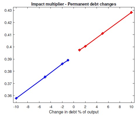
Note: Impact of the fiscal multiplier for the permanent change in debt experiment as a function of the size of the variation of government expenditure (as a % of GDP). The blue line corresponds to government expenditure contractions; the red line represents expansions.
Source: Brinca et al. (2023).

Finally, Brinca et al. (2023) show that the key mechanism, which relies on the differential response of labour supply across the wealth distribution as well as on movements of that same distribution, survives the introduction of nominal rigidities. They repeat the experiments in a state-of-the-art HANK model as in Auclert et al. (2021) and find the same pattern of fiscal multipliers that are increasing with the size of the government spending shock. The results and mechanism are the same for both deficit and balanced budget fiscal experiments.

A number of studies relate to the work done by Brinca et al. (2016), Brinca et al. (2021) and Brinca et al. (2023). Carroll et al. (2017) study the impact of the wealth distribution on the marginal propensity to consume. They measure marginal propensities to consume for a large panel of European countries and then calibrate a model for each country using net wealth and liquid wealth. The authors find the same type of relationship as documented by Brinca et al. (2016) for output multipliers: the higher the proportion of financially constrained agents in an economy, the higher the consumption multiplier.

Among empirical studies of fiscal multipliers, Ilzetzki et al. (2013) argue that multipliers are: (i) larger in developing countries than developed ones, (ii) larger under fixed exchange rates but negligible otherwise, and (iii) larger in closed economies than in open ones. The results in Auerbach and Gorodnichenko (2011) indicate that for a large sample of OECD countries, the response of output is large in recessions but insignificant during normal times. Anderson, Inoue, and Rossi (2016) find that in the context of the US economy, individuals respond differently to unanticipated fiscal shocks depending on age, income level and education. Blanchard and Leigh (2013) and Blanchard and Leigh (2014) find that during the sovereign debt crisis in Europe, the implemented fiscal consolidation programmes had a recessive effect on output and show that this effect is underestimated by the IMF. Alesina et al. (2015) find that tax-based consolidations lead to longer and deeper recessions than spending-based consolidations. Huidrom et al. (2020) find that the fiscal position plays a crucial role in shaping the magnitude of fiscal multipliers. Specifically, the estimated multipliers are consistently lower when government debt levels are elevated

Brinca et al. (2016) points out that in closed economies, government debt has the effect of crowding out physical capital, leading to a rise in the real interest rate. This elevation of the real interest rate causes an increase in the net present value of shocks affecting current income and thus larger fiscal multipliers from current income shocks. Conversely, it leads to a decrease in the net present value of shocks impacting future income and, thus, to smaller fiscal multipliers from these shocks. In small open economies, we may not see the same effect. However, there are reasons to believe that even in small open economies, debt would affect prices. For example, Chakraborty et al. (2017) document that, across countries, a disproportionate amount of commercial debt is held by nationals, and in the presence of some form of home-equity bias, a reduction in government debt could have real effects in the economy.

See Table 6 in the appendix for a comparison of debt and wealth levels in advanced economies.

.

Among quantitative macro papers studying the determinants of fiscal multipliers, Heathcote (2005) studies the effects of changes in the timing of income taxes and finds that tax cuts can have large real effects and that the magnitude of the effect depends crucially on the degree of market incompleteness. Hagedorn et al. (2019), in a New Keynesian model, present further evidence of the relevance of market incompleteness in determining the size of fiscal multipliers. Ferriere and Navarro (2020) provide empirical evidence showing that in the post-war U.S., fiscal expansions are only expansionary when financed by increases in tax progressivity. Finally, Krueger, Mitman, and Perri (2015) conduct a case study of the recent U.S. recession in a business-cycle model with infinite horizon. They find that the presence of wealth-poor individuals is important for the response of macroeconomic aggregates to the business-cycle shock.

In this section, we discuss the implications of the recent economic literature on the determinants of fiscal multipliers for fiscal policy in the Nordic countries, taking their economic characteristics into consideration. We conclude by using the results in Brinca et al. (2021) to obtain estimates of fiscal multipliers from fiscal consolidation in the Nordic countries.

Fiscal multipliers are significantly affected by income and wealth inequality due to their effect on low-wealth and credit-constrained consumers. The Nordic countries are notable for their significant levels of wealth inequality but low income inequality, see Table 3

See also Guvenen et al. (2022) for measures of income inequality across countries and changes over time. Many developed countries have recently experienced large increases in inequality. Notably, Norway, Denmark and Sweden stand out as countries with low income inequality and relatively modest growth in income inequality over time.

. The implication of this, perhaps somewhat dependent on the underlying reasons for the low income inequality and high wealth inequality, is that there will be a large fraction of low-wealth and credit-constrained consumers in the economy. Brinca et al. (2016) find that when they calibrate their model to match the wealth distribution of different OECD economies and allow, among other factors, the pension system and heterogeneous discount factors to vary across countries, the countries with more unequal wealth distributions have more low-wealth consumers. If higher income inequality is at least partially driven by idiosyncratic income risk, then the implication is that greater income inequality leads to more precautionary savings and fewer low-wealth consumers close to the borrowing constraint. Since the Nordic countries have high wealth inequality and low income inequality, both of these features point in the direction of large numbers of low-wealth consumers. Indeed, Table 4, which is reproduced from Brinca et al. (2016), shows that in a sample of 15 OECD countries, Sweden stands out as the single country with the lowest cumulative share of wealth in the bottom deciles. Finland also has a relatively low share of wealth in the bottom wealth deciles

For comparison, Table 7 in the appendix displays cumulative wealth distributions from Davies et al. (2017). In a sample of 15 OECD countries, Denmark and Norway have the least wealth concentrated in the bottom deciles of the wealth distribution.

.

Table 4. Cumulative distribution of net wealth

Note: Cumulative distribution of net wealth (variable: DN3001) from HFCS. For Canada, Japan, Sweden, the UK and the US, data is from the Luxembourg Wealth Study (LWS) Database (2015). For Switzerland, Davies, Sandstrom, Shorrocks, and Wolff (2011).

Having established that the Nordic economies have a large fraction of low-wealth consumers, the implication is, according to Section 3, that the fiscal multipliers from programmes that affect consumers’ current income will be high, and the fiscal multipliers from programmes that affect their future income will be low in the Nordic countries. This means that the effect of policies such as the Bush tax rebate cheques of 2001 and 2008, when taxpayers received cheques in the mail, should be large in the Nordic countries. On the other hand, the effects of a fiscal consolidation programme running over many years should be smaller in the Nordic economies than in the average OECD economy. We can use the empirical study by Brinca et al. (2021) to obtain estimates for the fiscal multipliers from fiscal consolidation in the Nordic countries after the 2008 financial crisis.

Brinca et al. (2021) take the seminal study by Blanchard and Leigh (2013) and show that the IMF forecast error for the fiscal multiplier from fiscal consolidation programmes was strongly correlated with income inequality. Using the regression results in Table 1 in Brinca et al. (2021), along with their inequality measures, we can obtain estimates of the fiscal multiplier in the Nordic countries (see the Appendix for a more detailed explanation of the approach). Table 5 shows the estimated fiscal multipliers for the Nordic countries, using different inequality measures, as well as the sample average.

Table 5. Calculations of fiscal multipliers

Note: Authors’ calculations.

We observe that the average estimate of the fiscal multiplier for 26 European economies is between 1.2 and 1.77, depending on which income inequality measure is used to augment the regression in Blanchard and Leigh (2013). These estimates are generally quite high, and it seems like the fiscal consolidation in Europe had a strong negative impact on the economy. By comparison, Brinca et al. (2016) find that the fiscal multiplier is in the 0.5–0.75 range for economies with high wealth inequality and close to 0 for economies with low wealth inequality when they replicate the SVAR exercise in Ilzetzki et al. (2013). Generally, the variation in fiscal multipliers has been observed to be quite large across time and place. However, the impact of fiscal consolidation in the Nordic countries is generally below the average due to low income inequality (the only exceptions are Iceland in the cases of the Y10/Y90 and Y2/Y98 shares). In Denmark, the multiplier is estimated to be in the 0.78-1.21 range, in Norway 0.86-1.35, in Sweden 0,88-1.41, in Finland 1.15-1.69, and in Iceland 1.18-1.69.

Recent research on the determinants of fiscal multipliers has established that they are highly state dependent, policy instrument dependent and size dependent. In particular, the income and wealth distributions are important for the effects of fiscal policy. In economies with high wealth inequality, we can expect to see larger fiscal multipliers from programmes that change consumers’ current income (such as direct transfers) and lower fiscal multipliers from policies that change their future income (such as debt consolidation programmes). In economies with higher income inequality, we can expect to see smaller fiscal multipliers from programmes that change consumers’ current income and larger multipliers from programs that change their future income. The mechanism goes through the labour supply elasticity across the wealth distribution. Low-wealth consumers are more responsive to current income shocks and less responsive to future income shocks. Economies with high wealth inequality or low income inequality are found to have many low-wealth consumers, and the aggregate labour supply elasticity is thus high with respect to current income shocks and low with respect to future income shocks.

The fiscal multiplier of government purchases is increasing in the spending shock, with more expansionary government spending shocks generating larger multipliers and more contractionary shocks generating smaller multipliers. This pattern is also caused by low-wealth consumers being more responsive to current income shocks and less responsive to future income shocks combined with the movement of the wealth distribution in response to current and future income shocks. An increase in government spending, financed by a negative shock to current income (lumpsum tax), shifts the wealth distribution to the left and increases the aggregate labour supply response to current income shocks. This leads to a fiscal multiplier that is increasing in the government spending shock. On the other hand, an increase in government spending, financed through a negative shock to future income (uptake of debt) shifts the wealth distribution to the right and thus increases the aggregate labour supply elasticity in response to future income shocks. This again leads to a fiscal multiplier that is increasing in the government spending shock.

The Nordic countries exhibit low income inequality but comparatively high wealth inequality. This duality in income and wealth distribution has important implications for the size of fiscal multipliers. The combination of high wealth inequality and low income inequality leads to a large fraction of low-wealth households. This implies that the fiscal multipliers from programmes that increase consumers’ current income, such as direct transfers, will be high, but the fiscal multipliers from programmes that change consumers’ future income, such as long-lasting fiscal consolidations, will be low in the Nordic countries.

Aiyagari, S.R., (1994). Uninsured idiosyncratic risk and aggregate saving. The Quarterly Journal of Economics, 109(3), 659-684.

Alesina, A., Barbiero, O., Favero, C., Giavazzi, F., & Paradisi, M., (2015). Austerity in 2009–13. Economic Policy, 30(83), 383-437.

Anderson, E., Inoue, A., & Rossi, B., (2016). Heterogeneous consumers and fiscal policy shocks. Journal of Money, Credit and Banking, 48(8), 1877-1888.

Auclert, A., Bardóczy, B., Rognlie, M., & Straub, L., (2021). Using the sequence‐space Jacobian to solve and estimate heterogeneous‐agent models. Econometrica, 89(5), 2375-2408.

Auerbach, A.J. & Gorodnichenko, Y., (2011). Fiscal multipliers in recession and expansion. In Fiscal Policy After the Financial Crisis (pp. 63-98). Chicago, Illinois: University of Chicago Press.

Baxter, M. & King, R.G., (1993). Fiscal policy in general equilibrium. The American Economic Review, 315-334.

Blanchard, O.J. & Leigh, D., (2013). Growth forecast errors and fiscal multipliers. American Economic Review, 103(3), 117-120.

Blanchard, O.J. & Leigh, D., (2014). Learning about fiscal multipliers from growth forecast errors. IMF Economic Review, 62(2), 179-212.

Blanchard, O. & Perotti, R., (2002). An empirical characterization of the dynamic effects of changes in government spending and taxes on output. Quarterly Journal of Economics, 117(4), 1329-1368.

Brinca, P., Faria-e-Castro, M., Ferreira, M.H., & Holter, H., (2023), January. The nonlinear effects of fiscal policy. Federal Reserve Bank of St. Louis working paper 2019-015F.

Brinca, P., Ferreira, M.H., Franco, F., Holter, H.A., & Malafry, L., (2021). Fiscal consolidation programs and income inequality. International Economic Review, 62(1), 405-460.

Brinca, P., Holter, H.A., Krusell, P., & Malafry, L., (2016). Fiscal multipliers in the 21st century. Journal of Monetary Economics, 77, 53-69.

Carroll, C., Slacalek, J., Tokuoka, K., & White, M.N., (2017). The distribution of wealth and the marginal propensity to consume. Quantitative Economics, 8(3), 977-1020.

Chakraborty, I., Holter, H. A., Hai, R., & Stepanchuk, S. (2017). The real effects of financial (dis)integration: A multi-country equilibrium analysis of Europe. Journal of Monetary Economics, 85, 28-45.

Davies, J. B., Sandstrom, S., Shorrocks, A., & Wol, E. N. (2007). Estimating the level and distribution of global household wealth, unu-wider research paper, nr. 2007/77. Retrieved from: https://www.wider.unu.edu/sites/default/files/rp2007-77.pdf.

Davies, J.B., Sandström, S., Shorrocks, A., & Wolff, E.N., (2011). The level and distribution of global household wealth. The Economic Journal, 121(551), 223-254.

Davies, J.B., Lluberas, R., & Shorrocks, A.F., (2017). Estimating the level and distribution of global wealth, 2000–2014. Review of Income and Wealth, 63(4), 731-759.

Devries, P., Guajardo, J., Leigh, D., & Pescatori, A. (2011). A new action-based dataset of fiscal consolidation. IMF Working Paper No. 11/128.

Domeij, D. & Floden, M., (2006). The labor-supply elasticity and borrowing constraints: Why estimates are biased. Review of Economic Dynamics, 9(2), 242-262.

Ferriere, A. & Navarro, G., (2020). The Heterogeneous Effects of Government Spending: It’s All About Taxes.

Guvenen, F., Pistaferri, L., & Violante, G.L., (2022). Global trends in income inequality and income dynamics: New insights from GRID. Quantitative Economics, 13(4), 1321-1360.

Gylfason, T., Holmström, B., Korkman, S., Söderström, H.T., & Vihriälä, V., (2010). Nordics in global crisis. Vulnerability and resilience. ETLA B.

Hagedorn, M., Manovskii, I., & Mitman, K., (2019). The fiscal multiplier (No. w25571). National Bureau of Economic Research.

Heathcote, J., (2005). Fiscal policy with heterogeneous agents and incomplete markets. The Review of Economic Studies, 72(1), 161-188.

Holter, H.A., Krueger, D., & Stepanchuk, S., (2019). How do tax progressivity and household heterogeneity affect Laffer curves? Quantitative Economics, 10(4), 1317-1356.

Huidrom, R., Kose, M.A., Lim, J.J., & Ohnsorge, F.L., (2020). Why do fiscal multipliers depend on fiscal Positions? Journal of Monetary Economics, 114, 109-125.

Ilzetzki, E., Mendoza, E.G., & Végh, C.A., (2013). How big (small?) are fiscal multipliers? Journal of Monetary Economics, 60(2), 239-254.

Jordà, Ò., (2005). Estimation and inference of impulse responses by local projections. American Economic Review, 95(1), 161-182.

Kaymak, B. & Poschke, M., (2016). The evolution of wealth inequality over half a century: The role of taxes, transfers and technology. Journal of Monetary Economics, 77, 1-25.

Krueger, D., Mitman, K. & Perri, F., (2016). Macroeconomics and household heterogeneity. Handbook of Macroeconomics ,2, 843-921. Elsevier.

Luxembourg Wealth Study (LWS) Database, (2015). Retrieved from: http://www.lisdatacenter.org. Luxembourg: LIS.

OECD (2022). Revenue Statistics 2022: The Impact of COVID-19 on OECD Tax Revenues, OECD Publishing, Paris, https://doi.org/10.1787/8a691b03-en.

OECD (2023). General government spending (indicator). doi: 10.1787/a31cbf4d-en.

Ramey, V.A. & Zubairy, S., (2018). Government spending multipliers in good times and in bad: evidence from US historical data. Journal of Political Economy, 126(2), 850-901.

Romer, C.D. & Romer, D.H., (2010). The macroeconomic effects of tax changes: estimates based on a new measure of fiscal shocks. American Economic Review, 100(3), 763-801.

Trabandt, M. & Uhlig, H., (2011). The Laffer curve revisited. Journal of Monetary Economics, 58(4), 305-327.

Vissing-Jørgensen, A. (2002). Limited asset market participation and the elasticity of intertemporal substitution. Journal of Political Economy, 110(4), 825-853.

To calculate the fiscal multipliers in Section 4 we proceed as follows. Brinca et al. (2021) estimate the below regression:

where is the forecast error in GDP growth from Blanchard and Leigh (2013),  is the planned fiscal consolidation from time to , is the inequality measure for country and  represents the mean of . They use lagged inequality measures to guarantee that it is not influenced by the GDP growth rate or the fiscal consolidation measures. Their regression results are reproduced below:

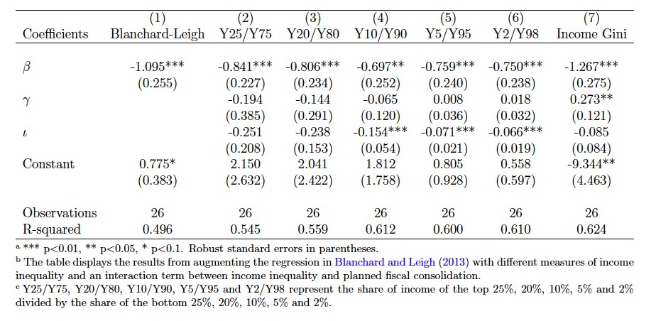
The IMF’s forecasted fiscal multiplier in Blanchard and Leigh (2013) is 0.5. It was, however, underestimated, and Brinca et al. (2021) find that the forecast error is correlated with income inequality. Thus, to obtain estimates of the country-specific fiscal multipliers, we simply add and  to 0.5, the value that was estimated as the average multiplier for all the countries prior to the 2008 crises by the IMF.

 

Table 7. Debt and wealth by country

Note: Data from Davies et al. (2017).

 Table 8. Cumulative wealth distributions

Note: Cumulative distribution of net wealth from Davies et al. (2017).