Nordic Economic Policy Review 2024
Automatic stabilisers in Iceland
Arnaldur Sölvi Kristjánsson
Abstract
This article studies the size of automatic stabilisation in the Icelandic tax-transfer system using administrative tax records. Automatic stabilisers – changes in public spending and revenue without active policy intervention – are generally considered to be an important component of stabilisation policies. It estimates the effects of shocks to income and employment on tax revenue and transfer payments. The tax-transfer system absorbs approximately 40% of an income shock and 60% of an unemployment shock. With some notable exceptions, estimated automatic stabilisers are relatively robust across different scenarios. The tax system is more important at higher income levels, whereas the unemployment insurance system is more important at lower income levels. By international comparisons, Iceland has a relatively high automatic stabiliser.
Keywords: automatic stabilizers; fiscal policy; income stabilization, demand stabilization
JEL Classification: E64, E62, H32, E63
1. Introduction
The three main functions of economic policy are allocation, stabilisation and redistribution (Musgrave and Musgrave, 1989). Stabilisation calls for policies that mitigate economic fluctuations, i.e. bring the economy closer to a balance as targeted by monetary and fiscal policy. The prevailing consensus suggests that, in the absence of major economic shocks, monetary policy should bear the main burden of stabilisation since the time lag in decision making and implementation is shorter for interest rate changes than changes in taxes and spending.
Fiscal policy can bring the economy closer to balance by boosting aggregate demand in a downturn and lowering it in an economic upswing. Economic stabilisation is the result of active decisions on tax and spending (discretionary fiscal policy) and from the automatic stabilisers. The latter refers to changes in public spending and revenue that are due to changes in economic activity and do not require active intervention by policy makers. In a downturn, unemployment goes up and income growth slows down, which automatically increases spending on employment related benefits and changes tax payments. The size of such effects depends on how tax and transfer payment systems are designed and how income changes. Automatic stabilisers should be smaller in a country with very strict eligibility requirements for unemployment benefit.
Like other trends in economics and politics, the pendulum swings over time. It is fair to say that following the financial crisis and the COVID-19 pandemic, the pendulum has swung in the direction of actively deploying fiscal policy in times of crisis. For example, Blanchard and Summers say that “Automatic stabilizers should be improved, and the scope for discretionary responses to adverse shocks should be revisited.” (2019: xiii).
In this paper, I use administrative tax records to report the results of the automatic stabilisers in Iceland, the tax records make it possible to accurately calculate tax payments for all taxpayers. I estimate the automatic stabilisers by investigating different shocks to market income and their effects on tax revenue and transfer payments. The effect of automatic stabilisers can be singled out by keeping everything else constant, including discretionary fiscal policy, monetary policy and behavioural changes. The paper follows the methodology used, among others, by Auerbach and Feenberg (2000) and Dolls et al. (2012).
To estimate the size and effects of the automatic stabilisers, I model shocks to income and employment. In the case of the income shock, market income changes either proportionally across the income distribution or in a manner that exacerbates inequality, e.g. income falls proportionally most for low-income individuals. As Iceland has a dual income tax system, whereby labour and capital income are taxed differently, the shock hits earnings first and then earnings and capital income. The unemployment shock only changes the number of individuals in work. The automatic stabilisers account for changes in tax payments and unemployment benefit caused by the shock.
The paper is organised as follows. Section 2 describes the concept of automatic stabilisers. Section 3 describes the measurements used. In section 4, the data and scenarios are described. The results are presented in section 5, and the final section presents some conclusions.
2 Automatic stabilisers
Automatic stabilisers are mechanisms built into the tax-transfer system that stabilise income and, as a result, stabilise consumption.
Automatic stabilisation can also be channelled through investment see e.g. Buettner and Fuest (2010), and Devereux and Fuest (2009).
In general, the larger the automatic stabilisers, the larger the public sector’s share of national income. Macro indicators such as revenue and expenditure to GDP ratios are sometimes used as a measure of automatic stabilisers (see, for example, Batini et al., 2014). The public sector is larger in Europe than in the US, for example, and the same applies to automatic stabilisers (Dolls et al., 2012).
The larger the automatic stabilisers, the smaller the effects of discretionary fiscal policy, i.e. fiscal multipliers are smaller. This is in accordance with standard Keynesian economics, as a larger share of any increased spending will end up as government revenue because a larger share of the increase in income is taxed. It is also in accordance with empirical evidence (see, for example, Mineshima et al., 2014). This means that countries with large automatic stabilisers will have less effective discretionary fiscal policies.
The components of automatic stabilisers on the spending side are primarily unemployment benefit and income-tested transfers. Such transfer payments increase automatically when income declines. Unemployment benefit and other employment-related transfer payments, e.g. social assistance, increase when a drop in income is due to higher unemployment. Income-tested transfers increase when income declines, whether it is due to unemployment or a drop in income.
The components of automatic stabilisers on the revenue side consist mainly of taxes. All taxes calculated as a percentage of income or consumption exhibit an element of automatic stabilisation. In the labour income tax schedule, higher earnings are taxed at the marginal tax rate, which usually increases with income. Hence, as income goes up by a certain percentage, post-tax income rises by a smaller percentage.
3 Measurement issues
The automatic response of the tax-transfer system measures the automatic sensitivity of net tax liabilities to changes in income.
See e.g. Musgrave and Miller (1948), Auerbach and Feenberg (2000), Dolls et al. (2012). The methodology followed here is described in Appendix A.
Imagine a proportional tax system under which all income is taxed at 40%. When income increases by 100 crowns, post-tax income increases by 60 crowns. This means that the tax system absorbs 40% of the growth in income. The same applies when income falls. When income goes down by 100 crowns, post-tax income only decreases by 60. Again, the tax system absorbs 40% of the change.
In a progressive tax system, the marginal tax rate exceeds the average tax.
In a progressive tax system the average tax rate, the share of income paid in taxes, increases with income. This can be done through increasing marginal tax rates, a tax threshold and tax credits. The average tax rate is the share of income paid in taxes. The marginal tax rate is the change in tax payments when income increases.
The size of the automatic stabiliser depends, therefore, on two factors. First, the average tax rate. The higher the average tax rate, the higher the automatic stabiliser. Second, the overall progressivity of the tax system. For the income stabilization coefficient it is the marginal tax rate that determine the size of the automatic stabiliser (Hutton and Lambert, 1979).
However, nominal amounts, tax thresholds and tax credits usually change at the turn of the year. If they go up proportionally with income, the average tax rate remains unchanged. This means that when income changes in a predictable manner, and the tax authorities increase nominal amounts at the same rate as income, the automatic stabilisation will be muted. The effects of the progressivity discussed above disappear. Only effects equal to the average tax rate remain.
Iceland has what is called a dual income tax system, like the other Nordic countries, which combines a progressive tax schedule for labour income with a low flat rate on capital income. The income stabilisation from capital income and labour income tax are defined as above. Since the capital income tax is lower and the labour income tax is progressive, the income stabilisation coefficient of the capital income tax is lower. The overall income stabilisation is a weighted average of both tax systems, where the weights are the share of the income component in overall income growth (Kristjánsson and Lambert, 2015). This means that the composition of income growth matters for the income stabilisation coefficient. When the share of capital income in the income growth is larger, the income stabilisation coefficient will be lower.
It is assumed that the tax incidence for taxes paid by employees is borne by employees. This assumption also covers employers’ social security contributions and pension contributions.
Evidence indicates that the majority of the incidence from social security contributions paid by employers falls on employees (for reviews, see Fullerton and Metcalf, 2002; Melguizo and González-Páramo, 2013).
For automatic stabilisers to stabilise aggregate demand, changes in current disposable income need to affect current consumption. People who are forward-looking will change their behaviour when changes in disposable income are permanent or their liquidity is constrained. The demand effect of temporary shocks depends on the frequency of liquidity constraints and to what degree individuals are forward-looking. Previous studies, such as those by Auerbach and Feenberg (2000) and Dolls et al. (2012), assumed that households facing liquidity constraints adjust expenditure proportionally to the changes in disposable income, whereas households without these constraints maintain consistent consumption levels. A different approach is taken in this article by making assumptions about the marginal propensity of consumption (MPC) for different income groups. The MPC is either assumed to be constant or to decrease with income.
4 Data and scenarios
I use a comprehensive administrative tax database containing the records of all Icelandic taxpayers, using their data for 2020. The dataset includes demographic information, which facilitates linking couples, as well as detailed individual income data. This data makes it possible to calculate tax payments and child benefit payments for all tax peyers. Notably, the Icelandic tax system has relatively few exemptions and exceptions, which facilitates highly accurate payment calculations for the entire population.
The tax and transfer components considered are:
- Labour income tax
- Capital income tax
- Child benefit
- Unemployment benefit
- Social security contributions
- Employers’ and employees’ pension contributions
- Value added tax
The labour income tax in Iceland has three brackets, up from two in 2019. The marginal tax rates ranged from 35.0% to 46.2% in 2020 (see Figure 1). Capital income is taxed at a marginal rate of 22% with a tax-free threshold. Rental income is taxed at 11%. Taxation on capital income is approximately 22% and proportional.
Child benefit is income-tested. As income goes up, child benefit goes down. The testing is based on household gross income. The reduction ranges from 4–10% for most households.
Figure 1. Marginal and average tax rates in Iceland, individuals with and without children, 2020.
Unemployed people have the right to unemployment benefit provided they worked enough hours in the year prior to becoming unemployed. Full entitlement equates to basic unemployment benefit for 30 months. In 2020, the amount was roughly 90% of minimum income. Individuals also receive income-related benefit for three months, which amounts to 70% of previous earnings up to a certain maximum, which amounts to 36% beyond minimum income.
Income-tested housing-related benefits are paid to tenants and homeowners, and these are not included in the analysis. The benefits paid to homeowners are rather low, excluding them only has a negligible effect on the results. The benefits paid to tenants are higher, but it is not possible to include them due to data limitations. However, as 79% of households where owner-occupied in 2022, this exclusion should not have a significant impact on the results (Statistics Iceland, 2024).
Employers pay a social security contribution, which is a tax, that amounts to 6.35% of earnings. Pension contributions are mandatory for employees and employers. The rates are 11.5% for employers and 4% for employees. These contributions entitle employees to a pension. The contributions are invested by pension funds. Although the payments do not constitute a tax, they are mandatory.
As per Dolls et al. (2012), I examine two types of shocks: an income shock and an unemployment shock. The income shock is based on data for 2020, while the unemployment shock is based on data for 2019, as explained below. The income stabilisation coefficient for the income shock is slightly higher in 2020 than in 2019 due to the 2020 tax reform. The difference is approximately 0.2 ppt.
4.2 Income shock
For the income shock, I start by considering a proportional change in market income of either -5% or +5% in 2020. That is, the income of all individuals goes either down or up by 5%. This income shock is applied to earnings alone and to both earnings and capital income, while unemployment benefit and social security remain unchanged during all income shocks.
In addition to proportional income changes, I also consider income changes that exacerbate inequality. The total change in income is the same as in the proportional income shock, either -5% or +5%. The change in inequality is such that the Gini coefficient of positive earnings increases by 3 Gini points (see Figure 2). According to Atkinson (2003), such a change constitutes an economically significant increase in inequality.
The Gini coefficient of positive earnings increases from 0.417 to 0.447. Bear in mind that this includes all individuals who receive any earnings in 2020. As many individuals only work part-time or part of the year, the Gini coefficient is quite large. In an international comparison, the earnings distribution of full-time earnings is compressed (see Eurostat, 2021). The post-shock income is MATEMATISK FORMULAR, where is pre-shock income and the average, and are parameters that are set such that overall income declines or increases by 5% and the Gini coefficient of positive income increase by 3 points.
Figure 2. The income shock scenarios.
4.3 Unemployment shock
I have modelled unemployment shocks in two separate ways. Firstly, I adopted the approach used by Dolls et al. (2012). This method of reweighting the proportion of unemployed people and symmetrically decreases the proportion in work. Individuals are defined as unemployed if they receive at least 10% of the basic unemployment benefit entitlement in 2019.
For the reweighting approach I present results for 2019. In 2020, many individuals received proportional unemployment benefits (hlutabætur) due to reductions in their hours worked. This was part of the government’s COVID-19 measures.
Secondly, I randomly make individuals of working age (24–69) unemployed and they receive unemployment benefit. Assuming their entitlement is 79% of the maximum, i.e. they receive 79% of the maximum unemployment benefit. This allows the income stabilisation coefficient to match the results obtained via the reweighting method. Increasing the entitlement percentage will increase the income stabilisation coefficient, as shown below. Individuals are assumed to be unemployed for the whole year, i.e. lose all earnings. Assuming that they only lose income for part of the year has a negligible effect on the income stabilisation coefficient.
5 Results
5.1 Individual-level income stabilisation
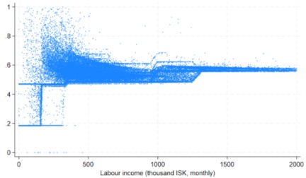
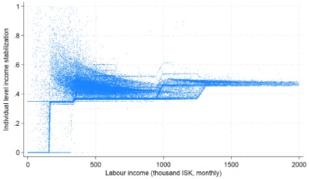
Before presenting the aggregate automatic stabilisers for the entire tax-benefit system, I begin by showing the individual-level automatic stabilisers. Figure 3 illustrates individual-level income stabilisation for a 5% proportional income decline. The definition of individual-level income stabilisation is the same as that of the aggregate income stabilisation coefficient, i.e. the change in net tax payments divided by the change in market income.
For most individuals, the individual-level income stabilisation coefficient closely follows the marginal tax rate schedule, which steps up incrementally at tax-bracket thresholds (at ISK 160, 340 and 950 thousand). However, there are deviations from the schedule, mainly driven by the joint taxation of cohabiting couples and joint income testing for child benefit.
Child benefit is income tested based on the sum of cohabiting couples’ incomes.
Joint income testing for child benefit can result in significant individual-level automatic stabilisers. When the income of a low-income individual falls by 5%, it leads to a minor change in child benefit in absolute terms. However, if the individual’s partner has a high income, the absolute change in the combined income of the couple can be substantial, causing a marked shift in child benefit, which can result in a very high automatic stabiliser for the low-income individual.
In Iceland, joint taxation applies to both the tax allowance and the top tax bracket. If an individual's income falls below the first tax bracket (income below ISK 150 thousand), the personal allowance is not fully utilised and can be applied to the partner if the joint income exceeds the tax threshold. When the incomes of both partners rise, the unused tax allowance diminishes, further increasing the individual-level stabilisation coefficient, which would not happen in a tax system without joint taxation. This also applies to the joint taxation of the top tax bracket, where the reduction in tax liabilities decreases as both partners’ incomes increase. This causes the income stabilisation both to increase and decrease (see further discussion in Section 5.2.).
Figure 3. Individual-level income stabilisation with a 5% proportional income decline.
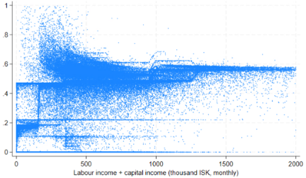
(a) Earnings increase
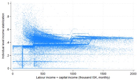
(b) Earnings and capital income increase
Transfer income remains unchanged. Individuals who only receive transfer income tax payments do not change. These individuals have an income stabilisation value of 0.
Other factors also contribute to deviations from automatic stabilisers based on the marginal tax rate schedule. Firstly, income-tested child benefit amplifies automatic stabilisers. Secondly, the municipal tax rate (útsvar) varies between municipalities. Thirdly, some individuals do not receive the full personal allowance and have a positive automatic stabiliser below the tax threshold.
Figure 3b shows the individual-level income stabilisation when earnings and capital income increase proportionally. Now, the individual-level stabilisation coefficient is below the marginal labour tax rate. As both earnings and capital income increase at the same rate, the income composition of each individual matters. The higher the share of capital income, the lower the individual-level income stabilisation.
5.2 Baseline results
In my baseline scenario, income changes proportionally by 5%, either affecting earnings alone or both earnings and capital income. Table 1 displays both proportional changes to income and changes that exacerbate inequality.
The aggregate size of the shock is approximately 5% in the inequality increasing shock.
Approximately 40% of a proportional income change is absorbed by the tax system. This percentage remains relatively consistent for both positive and negative earnings shocks. Since capital income remains unchanged during earnings shocks, labour income makes up 100% of the income growth, and the automatic stabiliser stems exclusively from labour income taxes and child benefit.
The income stabilisation coefficient attributed to child benefit constitutes only a small proportion of the overall impact. Child benefit is subject to income testing, meaning it is reduced as income rises, which makes the automatic stabiliser larger. However, the benefit reduction rate is notably lower than the marginal tax rate, and not all individuals have dependent children. Consequently, the child benefit system absorbs a significantly smaller portion of the income shock than the labour income tax.
Income changes that increase inequality produce an asymmetric effect on the automatic stabilisers. Such changes lead to a lower (higher) income stabilisation coefficient in the case of an income decline (increase) of approximately 5 ppt. The more inequality increases, the greater the effect on the income stabilisation coefficient. When income declines and increases inequality, a relatively larger proportion of the income change is borne by those on lower incomes, for whom marginal tax rates are lower. The opposite is the case in the event of an increase in income.
Capital income is taxed at a marginal rate of 22%, whereas labour income is taxed at marginal rates ranging between 35% and 46%. Consequently, when both labour and capital income go up or down, the tax system absorbs a smaller portion of the income shock related to capital income.
The income stabilisation coefficient for the capital income tax quantifies the proportion of capital income tax changes absorbed by the tax system. This figure is approximately 19% for proportional income changes, slightly below the marginal tax rate of 22%, due to a tax threshold in the capital income tax system and to the lower rate on rental income.
The income stabilisation coefficient for the labour income tax remains unchanged compared to an income shock that only affects earnings. The overall coefficient is a weighted average, with the weight being the proportion of income growth attributable to labour income. Given that labour income represents the largest share of income growth, the difference in the automatic stabilisation is not large (less than 2 percentage points).
Table 1. Income stabilisation coefficients from an income shock
Earnings change | Earnings and capital income change | |||||||
Proportional change | Increases inequality | Proportional change | Increases inequality | |||||
Decrease | Increase | Decrease | Increase | Decrease | Increase | Decrease | Increase | |
Total | 38.1% | 38.3% | 32.3% | 44.0% | 36.7% | 36.9% | 32.1% | 42.0% |
Labour income | 36.7% | 37.1% | 31.4% | 43.3% | 36.7% | 37.1% | 31.4% | 43.3% |
Capital income | - | - | - | - | 19.2% | 19.3% | 19.2% | 19.3% |
Labour income share | 100.0% | 100.0% | 100.0% | 100.0% | 92.3% | 92.3% | 92.2% | 91.9% |
Child benefit | 1.4% | 1.3% | 1.8% | 0.7% | 1.3% | 1.2% | 1.7% | 0.7% |
The labour income share is the share of total income growth due to labour income.
The results in Table 1 are based on calculations in which the share of income growth between labour and capital income is equal to its pre-shock status. Nevertheless, there is a substantial degree of variability in the proportion of income growth attributed to capital income. In recent decades, there have been many years when more than 50% of income growth has been attributable to capital income, although the share is much lower on average. Table 2 shows income stabilisation coefficients with different shares of labour income in income growth. The lower the share, the lower the income stabilisation coefficient.
Table 2. Income stabilisation income shock, different labour income shares in income growth
Labour income shares in income growth | Proportional income decrease |
50% | 28.0% |
60% | 29.7% |
70% | 31.5% |
80% | 33.2% |
90% | 35.0% |
100% | 36.7% |
Two different methods of estimating the income stabilisation coefficient for an unemployment shock are presented in Table 2. Firstly, using a reweighting method, increasing the weight of unemployment. Secondly, a random increase in unemployment, so that earnings plummet to zero and unemployed people receive unemployment benefit instead. The results presented are for three different increases in the unemployment rate, ranging from 2.5 to 10 percentage points.
The stabilisation coefficients from the unemployment shock are significantly larger than for the income shock: roughly 60%. In other words, around 60% of the fall in market income when unemployment goes up is absorbed by the tax-transfer system.
Over half of the stabilisation from the tax-benefit system in the wake of an unemployment shock is down to the unemployment benefit system. From the total stabilisation coefficient of roughly 60%, around 30–40% is due to the unemployment benefit system. By contrast, stabilisation via the labour income tax is much lower in the event of an income shock. Unemployment benefits are taxable, so part of the increase in the benefits is taxed. This explains the low proportion of the stabilisation coefficient that is down to the labour income tax.
Table 3. Income stabilisation coefficients from an unemployment shock
Random increase in unemployment | Reweighting unemployment share | |||||
2.5 ppt increase | 5 ppt increase | 10 ppt increase | 2.5 ppt increase | 5 ppt increase | 10 ppt increase | |
Total | 60.6% | 60.8% | 60.8% | 60.8% | 60.8% | 60.8% |
Labour income | 22.9% | 22.7% | 22.7% | 27.5% | 27.5% | 27.5% |
Capital income | - | - | - | 19.2% | 19.2% | 19.2% |
Labour income share | 100% | 100% | 100% | 86.6% | 86.6% | 86.6% |
Child benefit | 1.1% | 1.1% | 1.1% | 3.1% | 3.1% | 3.1% |
Unemployment benefit | 36.6% | 37.0% | 37.0% | 31.3% | 31.3% | 31.3% |
The estimates for income stabilisation coefficients are arrived at using the same methodology as Dolls et al. (2012). They estimated stabilisation coefficients for income and unemployment shocks for Europe and the USA. The stabilisation coefficients for an income shock are 26.3% for Europe and 24.4% for the USA. The coefficients are substantially larger, around 40% in Sweden and Finland and even higher in Denmark at 56%. The coefficients for Iceland are large by international comparison and in line with those of the Nordic countries.
Comparing the stabilisation coefficients for the unemployment shock, a similar picture emerges. The coefficient is substantially higher in Europe (48.5%) than in the USA (37.7%). The coefficients are substantially larger in the Nordic countries, ranging between 51.9% and 82.3%. This should come as no surprise as Iceland has a comparatively generous unemployment insurance system, like the Scandinavian countries.
According to OECD data, the Nordic countries score rather highly in the proportion of previous income paid as unemployment benefit, depending on the length of time unemployed.
In Iceland, joint taxation slightly lowers the estimated income stabilisation coefficient, with a minimal difference of less than one percentage point (see Table 4). Joint taxation operates in two ways. Firstly, it allows the transfer of unused personal allowances between partners. As a result, when both partners’ incomes rise, the unused portion of the allowance falls, which marginally increases the income stabilisation coefficient. Secondly, joint taxation is also allowed in the highest tax bracket. The tax relief from this depends on the combined incomes of both cohabitees. Under the current rules, an increase in both partners’ incomes can either raise or lower the tax deduction.
The tax deduction depends on the minimum of: (1) the difference between the income tax base of a higher-income individual and the upper threshold limits. (2) Half of the difference between the upper and lower threshold limits. (3) Half of the difference between the upper threshold limits and the income tax base of a lower-income individual. See Ministry of Finance and Economic Affairs (2019).
Table 4. Income stabilisation coefficients without joint taxation
Earnings decrease | Earnings and capital income decrease | Unemployment increases (5 ppt) | ||||
Proportionally | Increases inequality | Proportionally | Increases inequality | Random | Reweight | |
Total | 38.4% | 32.8% | 37.0% | 31.7% | 60.8% | 61.2% |
Labour income | 37.0% | 31.0% | 37.0% | 31.0% | 22.7% | 27.9% |
Capital income | - | - | 19.2% | 19.2% | - | 19.2% |
Labour income share | 100.0% | 100.0% | 92.3% | 92.2% | 100.0% | 86.6% |
Child benefit | 1.4% | 1.8% | 1.3% | 1.7% | 1.1% | 3.1% |
Unemployment benefit | - | - | - | - | 37.0% | 31.3% |
5.3 Changes in nominal amounts
Under the Icelandic tax system, nominal income amounts, tax thresholds and the personal allowance increase by 1% in real terms at the turn of the year. In all of the shocks outlined above, tax thresholds remain unchanged. One interpretation of this is that the shock is greater than the threshold increases from year to year. As a result, a positive income shock shifts individuals from lower to higher tax brackets. As discussed in Section 3, the stabilisation coefficient depends on the average tax rate and progressivity, i.e. the change in the average rate when income changes. When changes to tax thresholds are proportional to the tax base, and there is a proportional change in all incomes, the average tax rate for all individuals remains unchanged.
If the tax base increases by 5%, all thresholds change by 5%.
The unemployment shock stabilisation coefficients change much less: they fall by 6-7 percentage points. Increasing the nominal amounts does not change the unemployment benefit payments. As the tax system accounts for a small share of the stabilisation coefficient in an unemployment shock, reducing automatic stabilisation by income tax has a smaller effect on the stabilisation coefficient.
Table 5. Income stabilisation coefficients, nominal amounts change proportionally to the tax base
Earnings decrease | Earnings and capital income decrease | Unemployment increases (5 ppt.) | ||||
Proportional | Increases inequality | Proportional | Increases inequality | Random | Reweight | |
Total | 26.8% | 21.9% | 26.2% | 21.7% | 53.9% | 55.0% |
Labour income | 25.4% | 20.1% | 25.4% | 20.1% | 15.8% | 20.8% |
Capital income | - | - | 19.2% | 19.2% | - | 19.2% |
Labour income share | 100.0% | 100.0% | 92.3% | 92.2% | 100.0% | 86.6% |
Child benefit | 1.4% | 1.8% | 1.3% | 1.7% | 1.1% | 3.1% |
Unemployment benefit | - | - | - | - | 37.0% | 31.3% |
5.4 Social security contributions and pension contributions
The sections above only refers to direct taxes paid by individuals. Here I add an income tax paid by employers, social security contributions. Mandatory pension contributions paid by employees and employers are also included here. Though they are not tax payments and generate rights to pensions, they are mandatory and are calculated in proportion to earnings just as tax payments. Assuming the incidence is borne by employees, social security and pension contributions increase the stabilisation coefficient. When social security contributions are included and pension contributions are not, the income stabilisation coefficient increases by less than 4 percentage points for an income shock even though the tax rate is 6.35%. Although the social security contribution absorbs part of the income shock, the contribution from other components falls because the market income is now defined as including the social security contributions.
When social security and pension contributions are both included, the effect on income stabilisation is larger. The income stabilisation increases by roughly 13 percentage points for an income shock and by 3-7 percentage points for an unemployment shock.
Table 6. Income stabilisation coefficients with social security and pension contributions
Earnings decrease | Earnings and capital income decrease | Unemployment increases (5 ppt.) | |||||||||
Proportional | Increases inequality | Proportional | Increases inequality | Random | Reweight | ||||||
Total | 50.9% | 46.7% | 48.8% | 44.9% | 67.8% | 64.1% | |||||
Labour income | 31.2% | 26.6% | 31.2% | 26.6% | 20.0% | 25.3% | |||||
Capital income | - | - | 19.2% | 19.2% | - | 19.2% | |||||
Labour income share | 100.0% | 100.0% | 93.4% | 93.3% | 100.0% | 87.5% | |||||
Child benefit | 1.2% | 1.5% | 1.1% | 1.4% | 0.9% | 2.9% | |||||
Unemployment benefit | - | - | - | - | 32.5% | 29.1% | |||||
Social security contr. | 5.4% | 5.4% | 5.4% | 5.4% | 5.8% | 6.1% | |||||
Pension contribution | 13.2% | 13.2% | 13.2% | 13.2% | 8.6% | 2.5% | |||||
When these results are compared with the income stabilisation coefficients in Dolls et al. (2012) for Europe and the USA, the difference between Iceland and other countries is less stark. This is because the share of social security contribution in tax revenues is high in Europe. The average income stabilisation coefficient in Europe is 49.7% and is 37.7% with social security contributions and 50.9% with social security and pension contributions. The income stabilization coefficient for an unemployment shock is however high in an international comparison, also when pension contributions are excluded.
5.5 Income stabilisation across the income distribution
In a progressive tax system, income stabilisation will be heterogeneous across the income distribution. Table 7 presents income stabilisation coefficients for individuals with below and above median income.
For an income shock, the stabilisation coefficient is higher above the median income due to higher marginal tax rates at higher income levels. The difference between the income groups will be higher as the marginal tax rates increase more as income grows. The difference between the income groups is slightly higher for an income shock that increases inequality.
The stabilisation coefficient for an unemployment shock is slightly higher for individuals with below median income. There is, however, a substantial difference in the decomposition. For individuals with below median income, unemployment benefit explains almost all of the stabilisation coefficient. The tax has almost no automatic stabilisation below the median income. Above the median income, the tax is around 40% of the stabilisation coefficient, and the unemployment benefit is around 60%.
Table 7. Income stabilisation coefficients for individuals above and below the median income
Earnings change | Earnings and capital income change | Unemployment increases (5 ppt.) Random increase | ||||||||
Proportional decrease | Increases inequality. decline | Proportional decrease | I Increases inequality decline | |||||||
Below | Above | Below | Above | Below | Above | Below | Above | Below | Above | |
Total | 31.9% | 39.1% | 27.8% | 36.8% | 31.4% | 37.5% | 27.7% | 34.8% | 82.2% | 58.3% |
Labour income | 29.7% | 37.8% | 26.9% | 34.4% | 29.7% | 37.8% | 26.9% | 33.4% | 9.7% | 24.3% |
Capital income | - | - | - | - | 10.0% | 19.7% | 10.0% | 19.7% | - | - |
Labour income share | 100.0% | 100.0% | 100.0% | 100.0% | 97.3% | 91.6% | 99.1% | 88.2% | 100.0% | 100.0% |
Child benefit | 2.3% | 1.3% | 1.0% | 2.4% | 2.2% | 1.2% | 1.0% | 2.1% | 1.4% | 1.0% |
Unemployment ben. | - | - | - | - | - | - | - | - | 71.2% | 33.0% |
The median is defined on the basis of gross income.
5.6 Demand stabilisation
This section presents demand stabilisation for different assumptions about the marginal propensity to consume (MPC). The demand stabilisation coefficients are lower than the income stabilisation coefficient unless the MPC is 1. The results are sensitive to the assumption about the MPC and whether the MPC is constant or heterogeneous across the income distribution. Table 8 shows demand stabilisation coefficients with MPC ranging from ¼ to 1 and for MPCs that are constant and heterogeneous across the income distribution, where MPC is higher in the lower income quintiles. Demand stabilisation coefficients are shown with and without the VAT.
Table 8. Demand stabilisation with different MPC
Earnings decline (5%, proportional) | Unemployment increases (5 ppt., randomly) | |||
MPC | Without VAT | With VAT | Without VAT | With VAT |
1, constant | 38.1% | 47.7% | 67.1% | 60.8% |
1/2, constant | 19.1% | 25.3% | 34.5% | 30.4% |
1/2, heterogeny. | 7.6% | 10.4% | 15.0% | 13.7% |
1/4 constant | 10.2% | 13.0% | 17.5% | 16.2% |
1/4, heterogeny. | 3.8% | 5.3% | 7.6% | 6.9% |
Heterogeneous along the income distribution, with MPC=1/2 on average: MPC1=1, MPC2=3/4, MPC3=2/4, MPC4=1/4 and MPC5=0, where 1 refers to the lowest income quintile and 5 the highest. Heterogeneous MPC=1/4 is: MPC1=1/2, MPC2=1.5/4, MPC3=1/4, MPC4=0.5/4, MPC5=5. Quintiles are defined on the basis of gross income.
The results reveal that with a uniform MPC, the demand stabilisation coefficients decrease proportionally to the MPC. For example, the demand stabilisation at an MPC of ½ is roughly half that at an MPC of 1. When the MPC decreases across income levels, the demand stabilisation is about half that of scenarios with a constant MPC. Higher-income groups absorb more of the overall income change than lower-income groups. In situations where the MPC falls with income, groups with a larger portion of the total income change have the lowest MPC.
5.7 Changes in unemployment benefit and tax rates
The main components of automatic stabilisation in Iceland are the income tax system and the unemployment insurance system. This section considers the effects of changes in the unemployment insurance system and tax system. Table 9 shows the effect of higher unemployment benefit, a higher entitlement ratio and higher marginal tax rates in all tax brackets. Changes in the unemployment insurance system will only affect automatic stabilisation for an unemployment shock. Increasing the marginal tax rate will affect automatic stabilisation both for income and unemployment shocks.
Table 9. Change in income stabilisation coefficient with changed unemployment benefit system and higher marginal tax rates
Higher unemployment benefit | Higher entitlement ratio | Higher marginal tax rate | ||||
Random unempl. incr. (5 ppt.) | Random unempl. incr. (5 ppt.) | Income shock (-5% prop.) | Random unempl. incr. (5 ppt.) | |||
+10% | + 1.8 ppt. | + 5 ppt. per 5 ppt. | + 1.5 ppt. | + 1ppt. per 1ppt. | + 1.0 ppt. | + 0.6 ppt. |
+50% | + 1.6 ppt. | + 10 ppt. per 5 ppt. | + 1.5 ppt. | + 5ppt. per 1ppt. | + 1.0 ppt. | + 0.6 ppt. |
+100% | + 1.4 ppt. | + 20 ppt. per 5 ppt. | + 1.5 ppt. | + 10ppt. per 1ppt. | + 1.0 ppt. | + 0.6 ppt. |
In the baseline scenario, the entitlement ratio is 79%, i.e. unemployed people receive 79% of the maximum benefit. Effects of increasing unemployment benefits by 10-50%, entitlement ratio by 5-20 ppt. and the marginal tax rate by 1-10 ppt. on the income stabilization coefficient, measured per 10% increase in unemployment benefits, per 5 ppt. increase in entitlement ratio and per 1 ppt. increase in the marginal tax rate, respectively. For example, upon increasing unemployment benefits by 50%, the effects on the income stabilization coefficient are divided by 5.
Increasing the unemployment benefit by 10% increases the income stabilisation coefficient slightly more than increasing the entitlement ratio by 5 ppt. The cost of these reforms is very similar when measured in terms of higher income stabilisation coefficients. Increasing the income stabilisation coefficient by 1 ppt. costs in both reforms approximately 1.6% of the outlay on unemployment benefit in 2019, or 0.1% of income tax revenue.
Raising the marginal tax rate increases income stabilisation for both income and unemployment shocks. As income tax is a larger factor for an income shock stabilisation, it has a larger effect on the income stabilisation coefficient for an income shock than an unemployment shock. Increasing the marginal tax rate will, however, generate higher revenue – substantially more than the increase in expenditure caused by higher unemployment benefit.
Labour supply and unemployment are assumed to remain unchanged under higher unemployment benefits and higher marginal tax rates.
6 Conclusion
The income stabilisation coefficient in Iceland is roughly 40% for an income shock and roughly 60% for an unemployment shock. These coefficients do not change dramatically when we consider different types of income and unemployment shocks. When income decreases in a way that changes inequality, income stabilisation coefficients are lower changes in inequality need however to be substantial for the effect to be significant. The higher stabilisation coefficient for unemployment shocks is explained by the unemployment insurance system. The capital income tax leads to a lower stabilisation coefficient because capital income is taxed at a lower and less progressive rate, but the overall effect on the automatic stabilisers is not large unless the proportion of the income growth made up of capital income is sufficiently large.
By international comparisons, Iceland has a relatively high income stabilisation coefficient. It is at a similar level to Denmark, Finland and Sweden, and higher than the European average. However, when social security and pension contributions are included, the coefficients in Iceland are similar to those in other European countries. When only social security contributions are included, and not pension contributions, the income stabilisation coefficients are smaller in Iceland than in the other Nordic countries.
When we analyse income stabilisation across income distribution, the difference between income groups is not large. However, there is a difference in the importance of the tax-transfer components. The tax system is more important at higher income levels, whereas the unemployment insurance system is more important at lower income levels. Finally, demand stabilisation coefficients are substantially smaller than income stabilisation coefficients unless the marginal propensity to consume is sufficiently large. Falling marginal propensity to consume from current income reduces demand stabilisation coefficients.
The effects of automatic stabilisation can be increased by changing the parameters of the unemployment system or the tax system. Raising unemployment benefits by 10% boosts the income stabilization coefficient in response to an unemployment shock from 60.8% to 62.6%. Implementing such a reform would approximately cost 0.2% of the income tax revenue collected in 2019.
References
Atkinson, A. B. (2003). Income Inequality in OECD Countries: Data and Explanations,Working Paper No. 881. Munich: CESIfo, Univ. Munich.
Auerbach, A. J., & Feenberg, D. (2000). The significance of federal taxes as automatic stabilizers. Journal of Economic Perspectives, 14(3), 37-56.
Batini, N., Eyraud, L., Forni, L., & Weber, A. (2014). Fiscal multipliers: Size, determinants, and use in macroeconomic projections. Technical Notes and Manuals. 14. International Monetary Fund.
Blanchard, O., & Summers, L. H. (Eds.). (2019). Evolution or revolution?: rethinking macroeconomic policy after the Great Recession. Cambridge, Massachusetts: MIT Press.
Buettner, T., & Fuest, C. (2010). The role of the corporate income tax as an automatic stabilizer. International Tax and Public Finance, 17, 686-698.
Devereux, M. P., & Fuest, C. (2009). Is the corporation tax an effective automatic stabilizer? National Tax Journal, 62(3), 429-437.
Dolls, M., Fuest, C., & Peichl, A. (2012). Automatic stabilizers and economic crisis: US vs. Europe. Journal of Public Economics, 96(3-4), 279-294.
Eurostat (2001). Earnings statistics, march. Eurostat Statistics Explained. Retrieved from: https://ec.europa.eu/eurostat/statistics-explained/index.php?title=Earnings_statistics#Distribution_of_earnings
Fullerton, D. & G. E. Metcalf (2002). Tax Incidence, in A. Auerbach and M. Feldstein (eds), Handbook of Public Economics, vol. 4, 1787–872. Amsterdam: Elsevier
Hutton, J. P., & Lambert, P. J. (1979). Income tax progressivity and revenue growth. Economics Letters, 3(4), 377-380.
Kristjánsson, A. S., & Lambert, P. J. (2015). Structural progression measures for dual income tax systems. The Journal of Economic Inequality, 13, 1-15.
Melguizo, A., & González-Páramo, J. M. (2013). Who bears labour taxes and social contributions? A meta-analysis approach. SERIEs, 4, 247-271.
Mineshima, A., Poplawski-Ribeiro, M., & Weber, A. (2014). Size of Fiscal Multipliers, in Cottarelli, C., Gerson, P. and Senhadji, A., eds., Post-crisis Fiscal Policy, 315-371. Cambridge, Massachusetts: MIT Press.
Ministry of Finance and Economic Affairs (2019). “Endurskoðun tekjuskatts og bótakerfa hjá einstaklingum og fjölskyldum”.
Musgrave, R. A., & Musgrave, P. B. (1989). Public finance in theory and practice. McGraw-Hill Kogakusa.
Musgrave, R. A., & Miller, M. H. (1948). Built-in flexibility. The American Economic Review, 38(1), 122-128.
Statistics Iceland. (2024). Heimili: Staða á húsnæðismarkaði eftir heimilisgerðum 2004-2022. Retrieved from https://px.hagstofa.is/pxis/pxweb/is/Samfelag/Samfelag__lifskjor__4_husnaedismal__0_stadaahusnaedismarkadi/LIF03215.px
Appendix A
Market income Y^M is defined as the sum of labour and capital income,
where L is earnings, wage income and self-employment income, and K is capital income, the sum of interest income, dividends, realised capital gains and rental income, K^R . Capital income other than rental income is denoted by K^O , where K=K^O+K^R .
Disposable income consists of market income minus net tax payments plus transfer payments,
where T are tax payments and B=B^u+B^S are transfers, B^u is unemployment insurance, and B^S other transfers, social security and income-tested transfer payments.
There are separate tax schedules for labour and capital income. Tax payments on labour are denoted by T^L\left(Y^T\right) , where Y^T=L+B-D is taxable income and D is deductions. Capital tax payments are denoted by T^K\left(K^R,K^O\right) .
Social security payments are paid by employers and are a linear function of earnings,
where t_s=6.35\% . Pension fund contributions in Iceland are paid by employees and employers. The total pension contribution is,
where T_E and T_R are the pension fund contributions of employees and employers, respectively,
where Y^P=L+B^u is the income from which pension contributions are payable, roughly earnings plus unemployment benefits, and t_E=4\% and t_R=11.5\% .
Government intervention is defined as net tax payments, i.e. G=T-B , which is a function of market income, socio-demographic characteristics (e.g. marital status, number of children and previous employment record), the parameters of the tax-transfers system and income.
For social security contributions and employers’ pension contributions, it is assumed that the incidence is born by employees. In practice, this implies that social insurance contributions and employers’ pension contributions are included in gross income, which is defined as,
Tax payments are then defined as,
Though pension contributions are tax payments, they are mandatory.
The income stabilisation coefficient is defined as the share of gross income change that the tax system absorbs,
where \Delta Y_i^M=\left(\lambda^L_i-1\right)L_i+\left(\lambda^K_i-1\right)K_i is the income shock for the individual, i as discussed in section 4, \left(\lambda^L_i-1\right) and \left(\lambda^K_i-1\right) is the relative size of the income shock on labour income and capital income, respectively. In the proportional income shock \lambda^L_i=\lambda^L and \lambda^K_i=\lambda^K are constants, whereas it depends on income in the inequality-changing income shock. In the unemployment shock, \lambda^L\in\left\lbrace0,1\right\rbrace , individuals either lose all their employment income or it remains unchanged, capital income remains unchanged, i.e. \lambda^K=1 .
The income stabilisation coefficient can be decomposed into six terms,
where \alpha=\frac{\sum_i\Delta L_i}{\sum_i\Delta Y_i^M} is the share of labour income in market income growth, and
- : income stabilisation coefficient for the labour income tax
\tau_L=\frac{\sum_i\Delta T^L_i}{\sum_i\Delta Y_i^{}} - : income stabilisation coefficient for the capital income tax
\tau_K=\frac{\sum_i\Delta T_i^K}{\sum_i\Delta K_i^{}} - : income stabilisation coefficient for the employer’s social security contribution
\tau_S=\frac{\sum_i\Delta T^S_i}{\sum_i\Delta L_i^{}} - : income stabilisation coefficient for pension contributions
\tau_P=\frac{\sum_i\Delta T^P_i}{\sum_i\Delta L_i^{}} - : income stabilisation coefficient for child benefit
\tau_{cb}=-\frac{\sum_i\Delta CB_i}{\sum_i\Delta Y_i^M} - : income stabilisation coefficient for unemployment benefit.
\tau_u=-\frac{\sum_i\Delta B^u_i}{\sum_i\Delta Y_i^M}
The effect of automatic stabilisers on overall demand depends on the effects of disposable income changes on consumption, i.e. the size of the marginal propensity to consume,
where C_i is consumption and a_i is the marginal propensity to consume. VAT tax payments are a linear function of the tax rate,
where t_c is the VAT rate.
The VAT rate is a weighted average of VAT rates. There are two VAT brackets in Iceland, 11% and 24%. Most goods are taxed at the higher rate, and some are VAT-exempt. The weighted average tax rate is the revenue from VAT as a proportion of consumption in the national accounts.
when the marginal propensity to consume is constant, i.e. a_i=a\forall i , then,
where \tau_c=\frac{\sum_i\Delta T^c_i}{\sum_i\Delta Y_i^M} is the income stabilisation coefficient from VAT.
Appendix B
Figure A.1. Individual-level income stabilisation for a 5% proportional income decline without joint taxation.
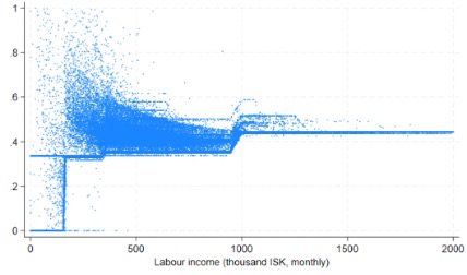
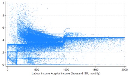
Figure A.2. Individual-level income stabilisation for a 5% proportional income decline without joint taxation. Only those without children.
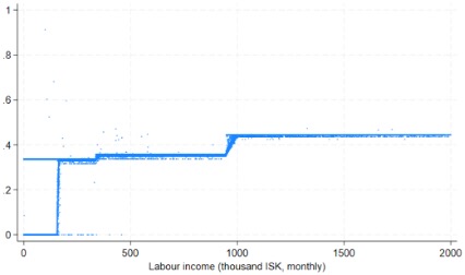
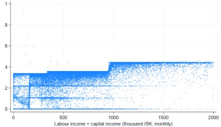
Figure A.3. Individual-level income stabilisation for a 5% proportional income decline, nominal amounts change proportionally to the change in income.
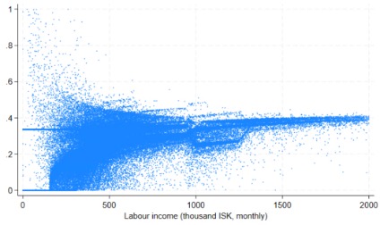
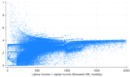
Figure A.4. Individual-level income stabilisation with social security and pension contributions for a 5% proportional income decline.