2. Method and data

The calculation of damage costs associated with emissions of SLCFs is adapted to data availability, especially considering comparability between the Nordic countries, and computational availability. In this chapter we first present the overall method for the calculations and present the data needed for the calculations. 

The calculation of total SLCF damage cost for a specific SLCF is made by multiplying the amount of emissions with the sum of unit climate effect given by a specific emission metric (Table 1) with the economic marginal climate damage cost for the specific pollutant and year (Figure 4) plus the other marginal SLCF damage costs (Table 3):

SLCF damage cost_{p,m,t,i} =E_{p,t}\times\left(CI_{p,m}\times CDC_{p,t,i}+ODC_{p,t,i}\right)

where:

SLCF damage cost (€₂₀₂₀/tonne pollutant)

E = emissions (kton)

CI = climate impact specified per SLCF (p) and per emission metric (m) (equivalent per tonne pollutant)

CDC = marginal climate damage cost specified per pollutant (p), year (t) and discount rate (i) (€₂₀₂₀ per equivalent)

ODC = marginal other damage cost specified per pollutant (p), year (t) and discount rate (i) (€₂₀₂₀ per tonne)

The calculations are made in Microsoft Excel.

The data used for this report consists of three parts. Nordic emissions of greenhouse gases and SLCFs, climate impact metrics to describe the effect on climate change of the emissions, as well assessments of economic externalities of climate change and air pollution.

The emission data and scenarios are for CO₂ taken from the latest available nationally reported emission data and scenarios to the European Environment Agency (EEA) for CO₂ (European Environment Agency, 2024c; 2024a), including gap filling made by EEA (Figure 1). All data are total emissions excluding effects of land use and land-use change and forestry (LULUCF).

Figure 1 Nationally projected CO₂ emissions as reported to the (European Environment Agency, 2024c) for the scenarios With Existing Measures (WEM) and With Additional Measures (WAM). Notice that only Finland and Sweden have reported WAM emission scenarios.

As can be noted, the scenarios registered by EEA are for different duration, where Norway stands out as only reporting CO₂-projections until 2035. Furthermore, only Sweden and Finland report low emission scenarios (WAM).

The SLCFs data is taken from the latest UNECE Air Convention policy brief produced by the Centre for Integrated Assessment Modelling (CIAM) and the Task Force on Integrated Assessment Modelling (TFIAM), which is used as negotiation support material during the ongoing revision of the UNECE Air Convention Gothenburg Protocol (CIAM and TFIAM, 2024). National scenarios for SLCFs were not used since they vary with respect to target year and the availability of high-policy-ambition emission scenarios, which makes them less relevant for policy support analysis. However, the scenarios produced by CIAM and TFIAM have undergone national consultation with official Nordic experts, and are checked against official statistics on fuel use, use of emission control technologies, as well as energy system fuel mixes etc. The emission scenarios from CIAM are presented in Figure 2 and Figure 3. As can be seen in the figures, the CIAM and TFIAM estimates indicate that there are substantial technical emission reduction potentials for all Nordic countries and all pollutants over the years. This potential can be seen through the comparison of the emissions in an air pollution policy baseline scenario (BSL) and a scenario in which all known emission control technologies are fully implemented (MTFR). The modelling and the scenarios suggest that Norway has the relatively largest emission reduction potential.

Figure 2 BSL and MTFR emission scenarios for the pollutants BC, PM2.5 and SO₂ (CIAM and TFIAM, 2024). In the figure, the values for the years 2020–2035 and 2045 are derived by interpolating the values for 2015, 2040, and 2050. When a line is not seen in the graph, the difference between BSL and MTFR is too small to be visible.

Figure 3  BSL and MTFR emission scenarios for the pollutants CH₄, NH₃, NMVOC, NO_x, and PM_other (CIAM and TFIAM, 2024). In the figure, the values for the years 2020–2035 and 2045 are derived by interpolating the values for 2015, 2040, and 2050.

The BSL and MTFR emission scenarios are not exactly similar to the nationally reported emission scenarios as they were reported in 2023. But they are similar enough for them to be useful for later policy recommendations. And as a reminder, these scenarios have been undergoing bilateral discussions with country representatives from the governments in the countries. In Appendix I to this report, we show a comparison between the BLE and the officially reported NFR emission projections to the Air Convention Centre for Emission Inventories and Projections (CEIP, 2023).

The climate impact of SLCF emissions is complicated to estimate and calculate. It also requires a large amount of computational power, a scarce resource despite fast growing computational capacity. In response to this, climate metrics are used to allow for quick comparisons and calculations of climate change effects of changes in emissions. In practice these metrics work as “exchange rates” to enable comparability between different types of emissions. The choice of which climate metric to use is largely dependent on political priorities and purpose of the analysis (Tanaka, Peters, and Fuglestvedt 2014). In the work leading to this report, we compiled data on several climate metrics and time horizons as presented in Table 1. Due to policy relevance, we have chosen to present results for the climate metric Global Warming Potential over a 100-year time horizon (GWP₁₀₀). As in Åström and Källmark (2023), we are normalising SCLF climate impact towards CH₄ emissions (CH₄-equivalents) since the climate characteristics of the long-lived and well-mixed greenhouse gas CO₂ are too different from poorly mixed and short-lived SLCFs like black carbon.

Table 1: Metric values for European SLCF emissions as CH₄-equivalences and CO₂-equivalences per pollutant and emission metric considered in the analysis. Due to lack of consistent data, values for SO₂ and NH₃ are for global emissions.

a: Own assumption that non-carbonaceous PM2.5 have RF identical to OC, b: Collins et al. (2013), c: Myhre et al. (2013), d: G. Myhre et al. (2013) supplementary material, e: D. T. Shindell et al. (2009)

To quantify the welfare effects of emissions of SLFCs one needs to calculate the marginal damage (external cost) of each pollutant that in the next step can be multiplied with tonnes or kilos of emissions for each of the Nordic countries (cf. the SLFC cost function above). We first present how marginal damage of climate change is valued (monetized), and then other marginal costs (e.g. diseases caused by air pollution).

Since climate change is a global problem and the damage of emissions are (almost) independent of where the emissions of greenhouse gases occur, the standard approach in cost-benefit analysis is to value (monetize) the climate change-related damage of an extra tonne of GHG emitted by estimates of the social cost of GHGs that is the same across countries (Dong, Tol, and Wang 2024; Ricke et al. 2018). The social cost of GHGs (SC-GHG) is defined as the “monetary value of the net harm to society from emitting a metric ton of that GHG into the atmosphere in a given year” (US Environmental Protection Agency, 2023). The SC-GHG is sometimes broken down into social cost of carbon (SCC, i.e. CO₂-specific), methane (SCM) and nitrous oxide (SCN) (US Environmental Protection Agency, 2023). This is because the damage from one tonne emitted of each of these GHGs has very different damage costs, due to e.g. lifetime in the atmosphere and a different temporal profile. As noted by US Environmental Protection Agency (2023), “In principle, SC-GHG is a comprehensive metric that includes the value of all future climate change impacts (both negative and positive), including changes in net agricultural productivity, human health effects, property damage from increased flood risk, changes in the frequency and severity of natural disasters, disruption of energy systems, risk of conflict, environmental migration, and the value of ecosystem services.” In practice, however, it has not been possible to date to calculate all these effects with a reasonable degree of certainty, so estimates of SC-GHG is often seen as conservative (negative effects are likely higher than positive of the ones that have not been included) (US Environmental Protection Agency, 2023). The damages that are now considered explicitly or implicitly represented by US Environmental Protection Agency (2023) are mortality and morbidity effects from heat/cold and extreme weather events, labor supply effects, energy consumption and production, loss of coastal land, buildings and infrastructure and effects on food production. In other words, there is no risk of double counting with those damage costs conventionally estimated for air pollutants. Many (most) of these effects are valued using adjusted market prices. Mortality effects are valued using estimates of the value of statistical life (VSL) of the USA, extrapolated to other countries in the world using GDP/capita adjustment (e.g. lower values in lower income countries).

It has not been possible in this report to update VSL estimates for the Nordic context. There is, however, work ongoing by the OECD to update their recommendations for which VSL values could be used for assessing mortality effects of policies (OECD, forthcoming).

Typically, SC-GHG is estimated using integrated assessment models, such as the well-known DICE (Nordhaus, 2017) and other models, sometimes combined with other methods, that integrate the climatic system with economic models.

Åström and Källmark (2023), that this report builds and extends upon, use estimates of SC-GHGs from the report by the US Interagency Working Group on Social Cost of Greenhouse Gases (2021). Since then, USEPA has built on that report and produced new SC-GHG estimates published in November 2023, that we use in the current report (US Environmental Protection Agency, 2023). The US Environmental Protection Agency (2023) presents annual estimates of SCC, SCM and SCN in USD 2020 from 2020 until 2080, with three alternative discount rates (2.5%, 2% and 1.5%). These rates are lower than in earlier guideline values, which corresponds well to newer research on discount rates (Rennert et al. 2022; Carleton et al., n.d.; P. H. Howard and Sterner, 2017).

We have extracted the relevant SCC-GHG (specifically SCC and SCM) numbers for each five-year period from 2020 to 2050, matching the years for our emission scenarios of the Nordic countries (USEPA 2013, Table A.5.1, Appendix 5, pages 154–155). USD 2020 amounts are converted to Euro 2020 using exchange rate of 0.876 ₂₀₂₀ per USD₂₀₂₀ as in Åström and Källmark (2023).

Note that the SC-GHG estimates are not presented with confidence bounds to account for uncertainty. Instead, they represent so-called certainty equivalents based on incorporating risk aversion,

Certainty equivalent of a risky cost (benefit) is the sure cost (benefit) that the consumer (i.e. in this case: society) considers just as good. Note that in many standard CBAs the decision maker is assumed to be risk neutral, in which case the certainty equivalent is just equal to the expected value. However, in the calculated SC-GHG, risk aversion is incorporated (see e.g. discussion in USEPA (2023, pages 73–76).

that can be used in cost-benefit analysis. These certainty-equivalents are based on an averaging of uncertainty (using e.g. Monte Carlo analysis) across the three damage modules.

USEPA (2023, p1): “The estimation process generates nine separate distributions of discounted marginal damages per metric ton – the product of using three damage modules and three near-term target discount rates – for each gas in each emissions year. These distributions have long right tails reflecting the extensive evidence in the scientific and economic literature that shows the potential for lower-probability but higher-impact outcomes from climate change, which would be particularly harmful to society. The uncertainty grows over the modeled time horizon. Therefore, under cases with a lower near-term target discount rate – that give relatively more weight to impacts in the future – the distribution of results is wider. To produce a range of estimates that reflects the uncertainty in the estimation exercise while also providing a manageable number of estimates for policy analysis, this report combines the multiple lines of evidence on damage modules by averaging the results across the three damage module specifications.”

Table 2 presents the resulting social cost of carbon (SCC) and social cost of methane (SCM) used in the calculations.

Table 2: Social cost of methane (SCM) and carbon (SCC) in €₂₀₂₀/tonne CH₄ and €₂₀₂₀/tonne CO₂

Although SCM is a more suitable metric than SCC, methane has a longer lifetime in the atmosphere and a different temporal profile (how long after an emission pulse that the temperature response occurs) than the other SLCFs. Since future values are discounted, it is reasonable to adjust the SCC values with respect to difference in temporal profiles. To do this we use the results from EPA (2023) and information from Figure 6.15 in Szopa et al. (2021) and the following assumptions:

The corresponding CH₄-normalised climate damage costs per tonne SLCF emissions are seen in Figure 4.

Figure 4: Social climate damage cost of one tonne of SLCF emissions emitted from the period 2015 to 2050 for the mid estimate of GWP₁₀₀ and with an initial discount rate of 2%.

Although this report is focused on assessing climate damage costs of SLCF emissions, the established damage costs of SLCF emissions are associated with health and environmental effects. To present a more complete picture of the total climate, health, and environmental damage cost of SLCF emissions, we complement the SLCF climate damage cost calculations with published data on other health and environmental damage costs of SLCF emissions. The latest and most authoritative estimate of these damage costs are published by the European Environment Agency (2024b). To enhance policy relevance, we utilise the damage costs as assessed when valuing effects on mortality with the value of a life year lost (VOLY) metric, just as was done by the European Commission in their presentation of a proposal for a revised NEC Directive (European Commission 2013). The alternative would be to use the metric value of statistical life (VSL) – as done when calculating the social cost of GHGs above. This is conceptually equally valid and allows for equal value being assigned to median persons as to elderly and weak persons. As a rule of thumb, the use of VSL instead of VOLY would render health and environmental damage costs to be a bit more than twice as high as when using VOLY (European Environment Agency, 2024b).

Table 3: Health and environmental damage costs of Nordic SLCF emissions from industrial sources in 2020

Since a large part of the health and environmental damage costs are estimated through the use of willingness-to-pay studies, it is important to adjust for increases in income for future years. In our work, we increase the health and environmental damage costs over time for the parts of the damage costs that is associated with willingness-to-pay (70% in 2020) in accordance with recommendations in (Atkinson et al. 2018). The increase corresponds to an assumed 2% growth in real income per year from the year 2020 until 2050, and a WTP-elasticity of 1.

We discuss the uncertainties related to the key hypotheses (called Key Claims) that typically motivate emission reduction measures, and serve as input to the most important knowledge gaps related to the results presented in this report. The main purpose of the uncertainty discussion is to provide input to potential needs for more knowledge on the input parameters used in the rest of the report. As a framework for the uncertainty analysis, we use as inspiration the guidance for lead authors in past IPCC Working Group 3 assessment reports (Mastrandrea et al. 2011). In the framework, the following dimensions are used to assess the validity of a finding: the type, amount, quality and consistency of evidence and the degree of agreement (Figure 5). When applicable in the IPCC work, this is then extended to express confidence (from “very low” to “very high”) and further to assign likelihood (from “exceptionally unlikely” to “virtually certain”) for quantifying the probability of an event. We focus the uncertainty discussion on air pollution and associated effects, since much of the climate change evidence is summarised in IPCC assessment reports etc.  

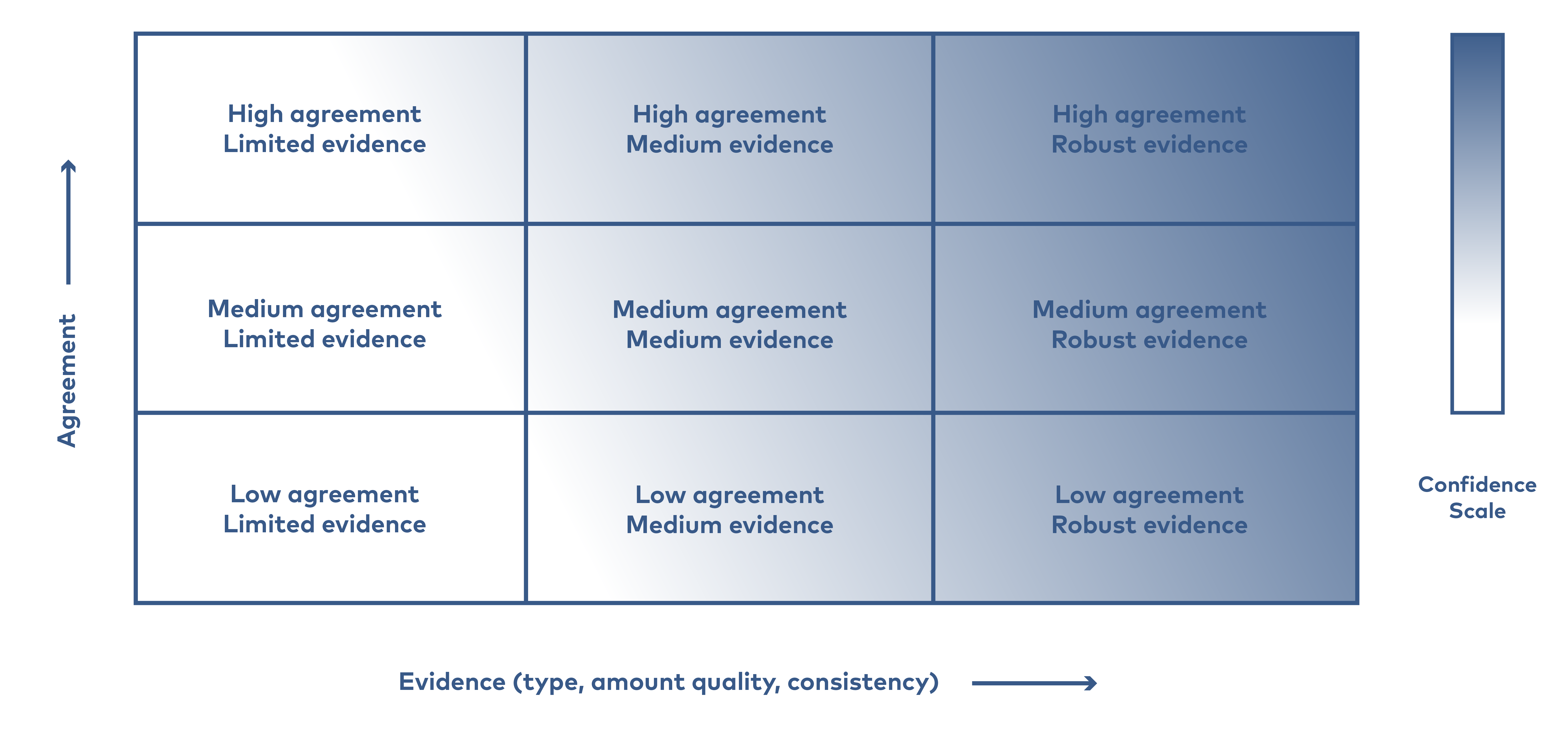
Figure 5: A depiction of evidence and agreement statements and their relationship to confidence. Confidence increases towards the top-right corner as suggested by the increasing strength of shading. Copied from Mastrandrea et al. (2011).

Through a joint project group discussion, we identified four key claims of relevance for air pollution aspects important for this report and its results. These key claims were then discussed regarding their robustness and the agreement of the scientific evidence supporting the claims.