
- Full page image w/ text
- Authors
- Table of contents
- Preface
- Terms and definitions used in this report
- Executive summary
- Sammendrag
- Introduction
- Background
- The Nordic Blue Carbon Project
- Chapter 1 – Distribution and biomass of blue forests in the Nordic countries
- Methods
- The Norwegian kelp dataset
- The Nordic kelp dataset
- Environmental variables used in the analyses
- Statistical models
- Estimating kelp area
- Estimating the production from Norwegian kelp
- Estimating the living biomass of Nordic kelp
- Seagrass distribution and living biomass
- Rockweed distribution and biomass
- Results and discussion
- Geographical distribution of Norwegian kelp
- Predicted areas of Norwegian kelp forests
- Geographical distribution of kelp forests in the Nordic countries
- Predicted areas of Nordic kelp forests
- Area estimates of Nordic seagrass
- Area estimates of Nordic rockweed
- Biomass of blue forests in the Nordic countries
- Conclusions
- Chapter 2 – Fieldwork on kelp carbon export and long-term storage of kelp carbon
- Methods
- Study area and sediment core sampling
- Sediment core processing
- Sediment dating (210 Pb)
- Total organic carbon, total carbon and chlorophyll a content in the sediment cores
- Sediment grain size analysis
- Species-specific qPCR assay development and core sample extraction
- 13C and 15N stable isotopes
- Export of dissolved organic carbon (DOC) from kelp
- Results and discussion
- Long-term storage (sequestration) of kelp POC in sediments
- Genetic analysis (quantitative qPCR)
- Stable isotopes
- Export of dissolved organic carbon (DOC) from kelp
- Conclusions
- Chapter 3 – Nordic blue carbon budget
- Methods
- Results and discussion
- Net primary production in the blue forest habitats
- Detritus formation and carbon export
- Sequestration of carbon in coastal areas and in the deep sea
- Updated carbon budget for Nordic blue forests
- Blue carbon at the science-policy interface
- Conclusions
- Chapter 4 – Blue forests now and in the future: pressures and management
- Methods
- Results and discussion
- Ecological interactions in Nordic blue forest ecosystems
- Interactions that influence the stability of Nordic blue forest ecosystems
- Environmental change and responses to pressures in Nordic blue forest
- Conclusions
- Chapter 5 - Policy recommendations
- References
- Appendix A
- Appendix B
- Appendix C
- About this publication
MENU

Blue Carbon – climate adaptation, CO2 uptake and
sequestration of carbon in Nordic blue forests
Results from the Nordic Blue Carbon Project
Helene Frigstad1
Hege Gundersen1
Guri S. Andersen1
Gunhild Borgersen1
Kristina O. Kvile1
Dorte Krause-Jensen2
Christoffer Boström3
Trine Bekkby1
Marc Angles d'Auriac1
Anders Ruus1
Jonas Thormar4
Kaya Asdal5
Kasper Hancke1
Contents
Preface
This is the final report of the 3-year project (2017–2019) “Blue carbon – climate adaptation, CO2 uptake and sequestration of carbon in Nordic blue forests" (the Nordic Blue Carbon Project) that has been led by the Norwegian Institute for Water Research (NIVA), in cooperation with GRID-Arendal, the Institute of Marine Research (IMR), Aarhus University and Åbo Akademi University. The project is funded by the Norwegian Environment Agency, through the Nordic Council of Ministers.
In 2017, the Nordic Blue Carbon Project published a report summarizing the results from the first year and the workshop “Status of knowledge for Nordic carbon cycling in blue forests” held at the Norwegian Environment Agency on 16–17 November 2017 (Frigstad et al., 2017).
On 21–22 November 2019, a final workshop for the Nordic Blue Carbon Project was held at the Norwegian Environment Agency. The workshop resulted in a policy brief summarizing the policy recommendations from the Nordic Blue Carbon Project, which was sent to relevant Nordic policy institutions and the relevant working groups under the Nordic Council of Ministers. The policy recommendations (included on p. 100) were written by Helene Frigstad, Hege Gundersen, Kasper Hancke, Guri S. Andersen, Trine Bekkby (all NIVA), Steven Lutz (GRID-Arendal), Jonas Thormar (IMR), Christoffer Boström (Åbo Akademi University) and Dorte Krause-Jensen (Aarhus University).
We thank Susanne Baden at the University of Gothenburg and Grethe Bruntse previously at Kaldbak Marine Biological Laboratory for sharing their datasets on macroalgae and seagrass. We are also grateful to Jacob Carstensen for extracting macroalgal data from the Danish marine monitoring program, and we thank the large number of field personnel from NIVA and IMR collecting the Norwegian kelp and seagrass datasets.
From NIVA, the following people are greatly acknowledged for providing assistance in the project: Solrun Figenschau Skjellum, Rita Næss, Eli Rinde, Hartvig Christie and Siri Moy.
Morten Foldager Pedersen (Roskilde University) and Karen Filbee-Dexter (University of Western Australia and Institute of Marine Research, Norway) are sincerely acknowledged for helping with the kelp incubation experiment for DOC production.
This final report presents the findings of the Nordic Blue Carbon Project over the period 2017–2019. A popular science summary of the results is presented in the Story Map, which can be found in the project web page.
Grimstad, 15 September 2020
Helene Frigstad
Project manager
Terms and defini|tions used in this report
Blue carbon – carbon captured by living organisms in coastal vegetated ecosystems (e.g. seagrass meadows, rockweed beds, kelp forests, salt marshes, and mangroves) and stored in biomass and sediments.
Blue carbon budget – in this report, an assessment of carbon cycle sources and sinks for blue forests (kelp, rockweed and seagrasses) in the Nordic region, through synthesis of information from literature and results from the Nordic Blue Carbon project.
Blue forests – in the Nordic Blue Carbon Project this includes the coastal vegetated ecosystems: kelp forests, seagrass meadows and rockweed beds.
Carbon export – the transfer of carbon between different carbon pools.
Carbon pool – the carbon stored in a specific species, ecosystem or geographic location.
Carbon uptake – a process by which the oceans (or plants on land) absorb carbon from the atmosphere.
Climate adaptation – in human systems, the process of adjustment to actual or expected climate and its effects, in order to moderate harm or exploit beneficial opportunities. In natural systems, the process of adjustment to actual climate and its effects; human intervention may facilitate adjustment to expected climate and its effects.
Climate change mitigation – a human intervention to reduce emissions or enhance the sinks of greenhouse gases (GHG).
Dissolved Organic Carbon (DOC) – the organic matter that is dissolved in seawater and is operationally defined as the fraction of carbon that passes through a filter (with pore size ranging from 0.22 to 0.70 micrometers).
Ecosystem services – ecological processes or functions with monetary or non-monetary value to individuals or society at large.
Greenhouse gas inventory – annual inventories of greenhouse gas emissions by sources and removals by sinks that are performed by individual nations according to reporting guidelines from the United Nations Framework Convention on Climate Change (UNFCCC).
Kelp forest – areas with a high density of kelp. In this report, more than 50% coverage of the species tangle kelp (Laminaria hyperborea) or sugar kelp (Saccharina latissima). In this study, oarweed (L. digitata) is also occasionally regarded as tangle kelp.
Living biomass – the amount of living organisms of a specific species or ecosystem.
Long-term storage of carbon – the long-term removal of carbon dioxide (CO2) or other forms of carbon from the atmosphere, with secure storage on climatically significant time scales (decadal to century). For particulate organic carbon (POC) this is defined as the carbon that is buried in the shelf or deep-sea sediments. For dissolved organic carbon (DOC) this is defined as the carbon transported below a water depth of 1 000m. Term used in Summary and Figures/Tables and equivalent to carbon sequestration.
Macroalgae – large algae attached to the bottom of the sea, such as tangle kelp, sugar kelp, and different species of rockweed.
Net primary production (NPP) – is defined as the difference between the energy fixed by plants and algae (incl. blue forest species) and their respiration, and is most commonly equal to the increment in biomass per unit surface and time. It is equivalent to the amount of organic material available to support consumers (herbivores and carnivores) in the food web.
Particulate organic carbon (POC) – the organic matter that is present in the form of particles and is operationally defined as the fraction of carbon that is retained in a filter (with pore size ranging from 0.22 to 0.70 micrometers).
Rockweed beds – in this study, beds of fucoid algae in the intertidal zone, mainly toothed wrack (Fucus serratus), bladder wrack (F. vesiculosus) and knotted wrack (Ascophyllum nodosum).
Seagrass meadows – beds of seagrass species, mainly eelgrass (Zostera marina).
Sedimentation – the particulate organic carbon (POC) that sinks out of the water column and settles in the coastal shelf or deep-sea sediments.
Sequestration – the long-term removal of carbon dioxide (CO2) or other forms of carbon from the atmosphere, with secure storage on climatically significant time scales (decadal to century). For particulate organic carbon (POC) this is defined as the carbon that is buried in the shelf or deep-sea sediments. For dissolved organic carbon (DOC) it is defined as the carbon transported below a depth of 1 000m. Term used in Chapters 1–4 and equivalent to long-term storage of carbon.
Sink – any process, activity or mechanism that removes carbon from the atmosphere.
Source – any process or activity that releases carbon into the atmosphere.
Sources: Glossary from IPCC Special Report on the Ocean and Cryosphere and Special Report on Global Warming of 1.5 °C
Executive summary
Nordic blue forests are coastal vegetated habitats, such as kelp forests, eelgrass meadows and rockweed beds, that are important natural sinks for carbon. Simultaneously, blue forests are at high risk from climate change and other human impacts, ranging from the effects of marine heat waves and increased frequency and intensity of storm events, eutrophication, coastal development and habitat fragmentation.
As highlighted in the IPCC Special Report on the Ocean and Cryosphere in a Changing Climate[1]IPCC Special Report on the Ocean and Cryosphere in a Changing Climate [H.- O. Pörtner, D.C. Roberts, V. Masson-Delmotte, P. Zhai, M. Tignor, E. Poloczanska, K. Mintenbeck, M. Nicolai, A. Okem, J. Petzold, B. Rama, N. Weyer (eds.)] (ipcc.ch/srocc) and the report by the High Level Panel for a Sustainable Ocean Economy[2]High Level Panel for a Sustainable Ocean Economy: The Ocean as a Solution for Climate Change: 5 Opportunities for Action (http://www.oceanpanel.org/climate), blue forests not only contribute to climate regulation, they also play an important role in climate adaptation. They provide a wide range of important ecosystem services such as benefits to local fisheries, enhance biodiversity, give storm protection, reduce coastal erosion, improve water quality and support local livelihoods.
Conservation and restoration of coastal vegetated ecosystems therefore represent nature-based climate solutions and a so-called “no-regret option” for mitigation and adaptation strategies, which are of benefit to a range of sectors, such as fisheries, trade, environmental protection and water management.
This report presents the main findings of the Nordic Blue Carbon Project (2017–2020) on the areal distribution and carbon budget of blue forests (kelp forests, seagrass meadows and rockweed beds) in the Nordic region. We have identified the main ecosystem effects of climate change and other human pressures on Nordic blue forests, tested the effect of moderating some of these pressures, and give scientific advice on management measures aimed at safeguarding these important coastal ecosystems for the future. Recently, there has been an increased focus on salt marshes as a blue forest habitat, however salt marshes were not covered in the Nordic Blue Carbon Project.
The Nordic Ministerial Declaration on Oceans and Climate[3]Nordic Ministerial Declaration on Oceans and Climate, 30.10.19 (www.norden.org/en/declaration/nordic-ministerial-declaration-oceans-and-climate) lays out the ambitions for increased Nordic collaboration on several areas that are highly relevant and compatible with the key findings and policy recommendations from the Nordic Blue Carbon Project.
First overall maps of blue forests in the Nordic region
The Nordic Blue Carbon Project has produced the first maps showing the areal distribution of blue forests for the Nordic region (Chapter 1). Kelp forests covered by far the largest area (around 11 000 km2) and were most widespread along the rocky shores of Norway, Iceland and the Swedish west coast. There were little to no kelp forests along the Swedish and Finnish coasts of the low-salinity Baltic Sea. Greenland has potentially large kelp forests, however the distribution of blue forest habitats could not be estimated due to limited data availability. Rockweed beds are found along most of the coastlines of the Nordic region (around 5 550 km2), however with low coverage in Denmark because of the mostly sandy or muddy seafloor. The areal distribution of seagrass (2 600 km2) was relatively small compared to kelp and rockweed, but still formed an important habitat along the coastlines of Sweden and Denmark.
Significant long-term storage of blue carbon in the Nordic region each year
Through a synthesized Nordic blue carbon budget, we estimated the long-term storage of carbon for blue forest habitats to 3.9 million tonne CO2 equivalents per year (1 087 Gigagram carbon per year). Greenland has been excluded from the estimates presented here due to lack of data. This represents an estimate of carbon permanently removed from the atmosphere each year by kelp forests, eelgrass meadows and rockweed beds in the Nordic region, and thereby the ability of these blue forest habitats to act as natural carbon sinks. The largest contribution to total Nordic long-term carbon storage was kelp forests (69%, 2.7 million tonne CO2 equivalents), followed by rockweed beds (19%, 0.8 million tonne CO2 equivalents) and finally seagrass meadows (12%, 0.5 million tonne CO2 equivalents). The Norwegian kelp forest alone contributed to 46% of the total long-term storage of carbon by blue forests in the Nordic region, due to the large areal distribution and high rates of carbon production and export.
These findings highlight the importance of Nordic blue forest habitats for long-term carbon storage in shelf and deep-sea habitats, accounting for around 1.8% of the total 2018 Nordic emissions (excluding LULUCF; UNFCCC). In addition to the annual long-term storage is a standing stock of living biomass that stores around 33 million tonne CO2 equivalents (9 236 Gigagram carbon). If all Nordic blue forests were to be lost, the net impact would be an immediate release of 33 million tonne CO2 to the atmosphere, as well as a reduced annual CO2 uptake (from the atmosphere) of 3.9 million tonne CO2.
The fluxes of blue carbon are not included in the national greenhouse gas inventories. However, this project has delivered the first step to providing a scientific basis for how this could be done should Nordic policymakers choose to report voluntarily on blue carbon. There are still considerable knowledge gaps that need to be addressed to reduce the uncertainties in the Nordic blue carbon budget and to report on these fluxes (see Chapter 3 and below).
Regardless of the potential for climate change mitigation, recent reports[4]IPCC Special Report on the Ocean and Cryosphere in a Changing Climate [H.- O. Pörtner, D.C. Roberts, V. Masson-Delmotte, P. Zhai, M. Tignor, E. Poloczanska, K. Mintenbeck, M. Nicolai, A. Okem, J. Petzold, B. Rama, N. Weyer (eds.)] (ipcc.ch/srocc) , [5]High Level Panel for a Sustainable Ocean Economy: The Ocean as a Solution for Climate Change: 5 Opportunities for Action (http://www.oceanpanel.org/climate) highlight that management measures to protect and restore blue forest habitats will have a wide range of societal and economical co-benefits, therefore making them “no-regret” mitigation options.
Developed eDNA method to identify kelp carbon in marine sediments
We have conducted fieldwork to address critical knowledge gaps in the Nordic blue carbon budget, focusing on the export and long-term storage of carbon from Norwegian kelp forests (Chapter 2). We developed a novel eDNA method for identifying and quantifying kelp in marine sediments, and for the first time documented the presence of tangle and sugar kelp in shelf sediments in Mid-Norway. This eDNA method will enable tracing of organic carbon from kelp and other macroalgae in seafloor sediments and thereby improve our understanding of the role of kelp and blue forests in the marine carbon cycle and their potential for long-term carbon storage. However, to adequately represent the geographical variation in kelp carbon storage within shelf and deep-sea areas of the Nordic countries, a great deal of knowledge is still needed.
Need to secure healthy blue forests today
We have analyzed the ecological relationships that are most important for maintaining healthy blue forest ecosystems. This has been done by creating network simulation frameworks based on qualitative ecological knowledge (Chapter 4). An important finding was that for all blue forest habitats, securing the resilience of blue forest systems today is the most important measure for safeguarding blue forests for the future. This involves continued efforts to limit additional human pressures from eutrophication, overfishing and habitat fragmentation.
To mitigate the negative effects of climate change on blue forests in the Nordic region and enhance the potential for long-term carbon storage, we found that improved light conditions would greatly increase the resilience of future kelp and rockweed habitats. For seagrass habitats, we found that reducing fishing pressure and nutrient loadings was the most effective measure for improving the long-term resilience. Relevant reports listing management measures that target these specific pressures are found in Chapter 4.
For all habitats, there was a strong negative impact from turf and other fast-growing algae that overgrow the key species and lead to unstable systems that are more vulnerable to climate change. One likely ecosystem response to climate change is in fact an increase in these fast-growing algal species. The simulations suggested that management measures aimed at securing robust and persistent mesograzer populations (small animals grazing on plants) are effective in securing the stability of these systems by facilitating natural control on turf algae and moderating the competitive relationship between turf algae and blue forests.
Knowledge needs for Nordic blue forests
As outlined in the Nordic Ministerial Declaration, there is an ambition to encourage and strengthen scientific research on natural carbon sinks in the Nordic region. The following knowledge needs for collaborative Nordic projects have been identified through the Nordic Blue Carbon Project:
Reduce uncertainties in the Nordic carbon budget and establish blue carbon inventories:
- Improved distribution mapping and monitoring of Nordic kelp, seagrass and rockweed habitats, by increasing field observations and cross-national access to environmental data layers for use in modelling (such as high-resolution data on depth and substrate). Greenland in particular represents a knowledge gap with potentially large areas of blue forests.
- Research targeted at reducing the main sources of uncertainty in the carbon budget, which include the rate of long-term storage of blue carbon in shelf and deep-sea sediments and the fate of dissolved organic carbon (DOC) that is exported out of the blue forest habitat.
- Knowledge exchange and collaboration between natural science researchers and policymakers, to develop IPCC guidelines for kelp forests.
- Further develop the knowledge basis to establish national greenhouse gas inventories for blue forest habitats.
- Basic research on the distribution and function of Nordic salt marshes.
Knowledge development on human pressures and effectiveness of management measures:
- Increase the understanding of human pressures on Nordic blue forests, especially multiple-driver relationships between effects of climate change and other human pressures (e.g. eutrophication, habitat fragmentation).
- Improve knowledge of ecosystem effects of overfishing (i.e. trophic cascade effects).
- Further develop management measures to implement new knowledge of ecosystem effects and their relative importance in improving the resilience of blue forest systems.
- Increase the knowledge on what determines restoration success in blue forest habitats, for example the role of connectivity and critical size of marine protected areas.
- Test, in the field, the effect of implementing management measures to improve the resilience of present-day blue forest habitats, for example by facilitating natural mesograzer control on turf algae using artificial refuges (reefs) and exerting varying degrees of urchin control.
- Map and develop measures to preserve areas of high sedimentation and long-term storage of carbon from blue forests in shelf and deep-sea sediments.
- Determine possibilities for using kelp cultivation to increase blue carbon biomass and its potential role in climate change mitigation.
Policy recommendations for Nordic blue forests
As an outcome of the Nordic Blue Carbon Project, the scientists involved outlined a set of policy recommendations based on their extensive expertise in the field. This group of scientists called for immediate and concerted policy actions to safeguard the Nordic blue carbon habitats, such as kelp forests, seagrass meadows and rockweed beds, especially through increased protection of coastal ecosystems by establishing marine protected areas and by strengthening the efforts to reduce human pressures, such as nutrient pollution, overfishing and habitat fragmentation. Today, there is enough scientific evidence to underpin the importance of these coastal ecosystems to support this call for action.
Footnotes
Sammendrag
Tittel: Blått karbon – klimatilpasning, CO2-opptak og sekvestrering av karbon i nordisk blå skog – endelig rapport 2017-2020
Nordisk blå skog omfatter kystnær fastsittende vegetasjon, for eksempel tareskog, ålegressenger og tangsamfunn, som alle er viktige naturlige karbonlagre. Samtidig er de blå skogene truet av klimaendringer og andre menneskeskapte påvirkninger, slik som marine hetebølger, økt hyppighet og intensitet av stormer, eutrofiering, overfiske, utbygging i kystområdene og habitatfragmentering.
FNs Klimapanels spesialrapport om hav og is[1]FNs klimapanels spesialrapport om havet og kryosfæren [H.- O. Pörtner, D.C. Roberts, V. Masson-Delmotte, P. Zhai, M. Tignor, E. Poloczanska, K. Mintenbeck, M. Nicolai, A. Okem, J. Petzold, B. Rama, N. Weyer (eds.)] (ipcc.ch/srocc) og Høynivåpanelet for bærekraftig havøkonomi[2]Høynivåpanelet for en bærekraftig havøkonomi (http://www.oceanpanel.org/climate) konstaterer at den blå skogen er viktig for regulering av klimaet, men fremhever også dens viktige rolle i vår tilpasning til klimaendringer. Blå skog bidrar til en rekke viktige økosystemtjenester ved å danne grunnlaget for fiskerier, biologisk mangfold, stormbeskyttelse, erosjonsbeskyttelse, vannrensing og lokal næringsvirksomhet i kystnære områder.
Bevaring og restaurering av blå skog vil være naturbaserte, såkalte «no-regrets»-løsninger for klimatiltak og -tilpasninger, og ha en positiv virkning for en rekke sektorer, som fiskeri, handel og miljø- og vannforvaltning.
Denne rapporten presenterer hovedfunnene fra blått karbon-prosjektet (2017-2020). Her vises for første gang heldekkende kart over områder med blå skog (tareskog, ålegressenger og tangbeltet) i den nordiske regionen. Rapporten presenterer også det første nordiske karbonbudsjettet for blå skog. Vi har identifisert økosystemeffektene av klimaendringer og andre menneskeskapte påvirkninger, og vi gir vitenskapelig baserte råd om forvaltningstiltak som kan bidra til å bevare disse viktige kystøkosystemene for fremtiden. Det er økende oppmerksomhet rundt saltmarsker (salt marshes) som en form av blå skog, men denne habitattypen var ikke inkludert i utlysningen av prosjektet.
Nordisk ministerråds erklæring om hav og klima[3]Det nordiske ministerråds erklæring om hav og klima, 30.10.19 (www.norden.org/en/declaration/nordic-ministerial-declaration-oceans-and-climate) presenterer ambisjonene for økt nordisk samarbeid på en rekke områder som er relevante for og sammenfallende med hovedfunnene og forvaltningsrådene fra dette prosjektet.
Det første helhetlige kartet over blå skog i den nordiske regionen
I denne rapporten presenteres de første heldekkende kartene over områder av blå skog i den nordiske regionen (kapittel 1). Tareskog dekker det langt største området (rundt 11 000 km2) og er mest utbredt langs kysten av Norge og Island og på den svenske vestkysten. Det er liten eller ingen tareskog langs den svenske eller finske kysten av Østersjøen, der vannet ikke er tilstrekkelig salt for tarevekst. Grønland har et stort potensial for tareskog, men på grunn av svært lite data fra dette området er estimatet av utbredelsen ikke sikkert. Tangbelter er vanlig langs mesteparten av den nordiske kystlinjen (rundt 5 500 km2), men er lite utbredt langs Danmark, siden det meste av havbunnen her består av bløt sand og mudder. Sammenlignet med tang og tare er utbredelsen av sjøgress (2 600 km2) relativt begrenset, men utgjør likevel et viktig habitat langs kysten av Sverige og Danmark.
Betydelig langtidslagring av blått karbon i den nordiske regionen hvert år
I det sammenfattede nordiske budsjettet for blått karbon anslo vi at rundt 3,9 millioner tonn CO2-ekvivalenter langtidslagres hvert år (tilsvarende 1 087 gigagram karbon per år). Dette er et estimat for hvor mye karbon som hvert år fjernes permanent fra atmosfæren av tareskog, ålegressenger og tangbeltet i den nordiske regionen, og er med andre ord et mål på den evnen blå skog har til å fungere som et naturlig karbonlager. Tareskogen ga det største bidraget til den samlede nordiske langtidslagringen av karbon (59%, 2,7 millioner tonn CO2-ekvivalenter), etterfulgt av tangbeltet (12%, 0,5 millioner tonn CO2-ekvivalenter) og ålegressengene (12%, 0,5 millioner tonn CO2-ekvivalenter). Den norske tareskogen bidro alene til 46% av langtidslagringen av karbon som finner sted i nordisk blå skog, på grunn av sin store utbredelse og høye rater av karbonproduksjon og -eksport.
Disse funnene understreker den betydningen nordisk blå skog har for langtidslagring på kontinentalsokkelen og i dyphavet, med en kapasitet på rundt 1,8 prosent av de totale nordiske utslippene i 2018 (unntatt LULUCF, jf. UNFCCC). I tillegg til å langtidslagre karbon absorberer også den stående biomassen i blå skog rundt 33 millioner tonn CO2-ekvivalenter (9 236 gigagram karbon). Hvis all nordisk blå skog skulle forsvinne, ville 33 millioner tonn CO2 frigis til atmosfæren. I tillegg ville den blå skogen ikke lenger ta opp 3,9 millioner tonn CO2 fra atmosfæren hvert år.
Fluksene av blått karbon er ikke inkludert i de nasjonale utslippsregnskapene, men dette prosjektet har tatt det første steget mot å levere det vitenskapelige grunnlaget nordiske beslutningstakere vil trenge for eventuelt å beslutte en frivillig rapportering på blått karbon. Det er fremdeles betydelige kunnskapsbehov og usikkerheter i budsjettet for nordisk blått karbon (se kapittel 3 og under).
Nylige rapporter[4]FNs klimapanels spesialrapport om havet og kryosfæren [H.- O. Pörtner, D.C. Roberts, V. Masson-Delmotte, P. Zhai, M. Tignor, E. Poloczanska, K. Mintenbeck, M. Nicolai, A. Okem, J. Petzold, B. Rama, N. Weyer (eds.)] (ipcc.ch/srocc),[5]Høynivåpanelet for en bærekraftig havøkonomi (http://www.oceanpanel.org/climate) fremhever at uavhengig av potensialet for utslippsreduksjoner vil forvaltningstiltak for å bevare og restaurere blå skog ha en rekke positive økonomiske og sosiale følger. Bevaring og restaurering av blå skog betraktes derfor som en såkalt «no-regrets»-klimaløsning.
Metode basert på miljø-DNA for identifisering av karbon fra tare i marine sedimenter
I prosjektet er det utført feltarbeid for å fylle kritiske kunnskapsbehov i budsjettet for nordisk blått karbon, med fokus på eksport og langtidslagring av karbon fra den norske tareskogen (kapittel 2). Vi har utviklet metodikk for å identifisere og kvantifisere tare i marine sedimenter ved hjelp av analyser av miljø-DNA, og har for første gang dokumentert sukkertare og stortare i sedimentprøver fra kontinentalsokkelen i Midt-Norge. Denne metoden gjør det mulig å spore organisk karbon fra tare og andre makroalger i bunnsedimenter, noe som vil bidra til økt forståelse av hvilken rolle tare og blå skog spiller i den marine karbonsyklusen og av potensialet for langtidslagring av karbon. Det er imidlertid fortsatt behov for mer data for å kunne dekke den geografiske variasjonen i karbonlagring fra tare i marine sedimenter i den nordiske regionen.
Behovet for å sikre blå skog i dag
Vi har analysert økologiske sammenhenger i blå skog, og identifisert hvilke forhold som bidrar sterkest til å opprettholde sunne økosystemer. Dette er gjort ved analyser av et stort antall nettverkssimuleringer basert på kvalitativ økologisk kunnskap (kapittel 4). Et sentralt funn var at det viktigste for å bevare blå skog for fremtiden er å sikre robuste (resilient) systemer i dag. Dette inkluderer tiltak for å begrense eutrofiering, overfiske og habitatfragmentering.
Den viktigste endringen som er nødvendig for å øke motstandsdyktigheten i fremtidige tare og tanghabitater og dermed begrense skadelige effekter av klimaendringer, er forbedrede lysforhold. For sjøgress fant vi at en reduksjon i fisketrykket og næringsbelastningen var de endringene som mest effektivt økte motstandsdyktigheten på lang sikt. En oversikt over relevante rapporter som identifiserer forvaltningstiltak spesifikt rettet mot å oppnå disse miljøforbedringene, er inkludert i kapittel 3.
En sterk vekst i lurv og påvekstalger (rasktvoksende, ofte trådformede alger som hindrer lys- og substrattilgang for tare, tang og sjøgress) fører til ustabile blå skoger og gjør dem mer sårbare for klimaendringer. Økningen i slike rasktvoksende algearter er en sannsynlig økosystemrespons på klimaendringer. Simuleringene tydet på at forvaltningstiltak som sikrer robuste og vedvarende bestander av mesobeitere (små beitende dyr), vil være effektive for å sikre motstandsdyktigheten i disse systemene. Mesobeitere utøver en naturlig kontroll på rasktvoksende alger og modererer dermed konkurranseforholdet mellom de rasktvoksende algene og den blå skogen.
Kunnskapsbehov for nordisk blå skog
Som fremhevet i erklæringen fra Nordisk ministerråd[6]Det nordiske ministerråds erklæring om hav og klima, 30.10.19 (www.norden.org/en/declaration/nordic-ministerial-declaration-oceans-and-climate), er støtte til og styrking av vitenskapelig forskning på naturlige karbonlagre i den nordiske regionen en ambisjon. De følgende kunnskapsbehovene for samarbeidsprosjekter i den nordiske regionen har blitt identifisert i dette prosjektet:
Redusere usikkerhet i budsjettet for nordisk blått karbon og etablere utslippsregnskap for blå skog:
- Forbedret arealkartlegging og overvåking av nordisk tare, ålegress og tang gjennom flere feltobservasjoner og bedre tilgang på miljødata for modellering på tvers av nasjoner (slik som høyoppløselige data på dybde og substrat). Kunnskapsgrunnlaget er spesielt svakt på Grønland, der det finnes et stort potensial for utbredelse av blå skog.
- Forskning for å redusere usikkerhetene i karbonbudsjettet, slik som anslagene over langtidslagring av blått karbon i marine sedimenter (på kontinentalsokkelen og i dyphavet) og av hva som skjer med løst organisk karbon (DOC) som eksporteres ut av blå skog.
- Kunnskapsutveksling og samarbeid mellom forskere og beslutningstakere for å utvikle IPCCs retningslinjer for tareskog.
- Videreutvikle kunnskapsgrunnlaget for etablering av nasjonale utslippsregnskap for blå skog.
- Grunnleggende forskning på utbredelsen av og funksjonen til nordiske saltmarshes.
Kunnskapsutvikling om effekten av menneskeskapt miljøpåvirkning og effekten av forvaltningstiltak:
- Øke forståelsen av hvordan menneskeskapte miljøendringer påvirker nordisk blå skog, spesielt effekter av samlet belastning av klimaendringer, eutrofiering og habitatfragmentering.
- Økt kunnskap om økosystemeffekter av overfiske (effekter av trofiske kaskader).
- Implementere ny kunnskap om økosystemeffekter i forvaltningstiltak med sikte på å øke de blå skogenes motstandsdyktighet.
- Økt kunnskap om hva som fører til vellykket restaurering av blå skog, for eksempel betydningen av romlig kontinuitet og minstestørrelse av marine bevaringsområder.
- Teste (i felt) effekten av forvaltningstiltak som tar sikte på å øke motstandsdyktigheten til blå skog, for eksempel gjennom å legge til rette for naturlig kontroll av rasktvoksende alger med mesobeitere (ved bruk av kunstige rev), og ved å utøve varierende grad av kontroll på kråkebollebestanden.
- Kartlegge og utvikle tiltak for å bevare områder med høy karbonlagring i marine sedimenter på kontinentalsokkelen og i dyphavet.
- Kartlegge mulighetene for å anvende tangdyrking til å øke biomasse av blått karbon som et mulig klimadempende tiltak.
Forvaltningsråd for nordisk blå skog
Forskerne i det nordiske blått karbon-prosjektet har utarbeidet et sett med forvaltningsråd basert på sine erfaringer, og oppfordrer til øyeblikkelige og samlede grep for å bevare de nordiske blå skogene. Tiltak for bevaring av marine økosystemer inkluderer opprettelse av marine verneområder og økt innsats for å redusere menneskelige påvirkningsfaktorer, slik som overgjødsling, overfiske og habitatfragmentering. Det finnes i dag nok vitenskapelig kunnskap om viktigheten av disse kystøkosystemene til å underbygge denne appellen.
Footnotes
- ^ FNs klimapanels spesialrapport om havet og kryosfæren [H.- O. Pörtner, D.C. Roberts, V. Masson-Delmotte, P. Zhai, M. Tignor, E. Poloczanska, K. Mintenbeck, M. Nicolai, A. Okem, J. Petzold, B. Rama, N. Weyer (eds.)] (ipcc.ch/srocc)
- ^ Høynivåpanelet for en bærekraftig havøkonomi (http://www.oceanpanel.org/climate)
- ^ Det nordiske ministerråds erklæring om hav og klima, 30.10.19 (www.norden.org/en/declaration/nordic-ministerial-declaration-oceans-and-climate)
Introduction
Background
Marine plants and algae take up inorganic carbon from the atmosphere and ocean through photosynthesis, and convert this carbon to biomass, thereby contributing to an oceanic carbon uptake from the atmosphere (terms marked in bold (on first use) are defined in the Terms and Abbreviations section). The Global Carbon Project estimates that around 23% of the anthropogenic emissions over the last decade have been absorbed by the ocean, and even small changes in this oceanic carbon uptake will have large consequences for the amount of CO2 remaining in the atmosphere and therefore on the global effects of climate change on nature and societies.
The biological uptake of carbon in coastal vegetated systems (e.g. seagrass meadows, rockweed beds, kelp forests, salt marshes, and mangroves) is referred to as blue carbon. How long this blue carbon remains in the oceans will vary, and the carbon bound in marine biomass can have several different fates after the organism dies. The carbon can be recycled in the water masses and a fraction released back to the atmosphere, while another fraction of the carbon will sediment on the seafloor (on coastal shelves or in the deep-sea sediments). Of this carbon that settles on the seafloor, an even smaller fraction will escape the recycling in the sediments and be sequestered (equivalent term: long-term storage of carbon) on climatically significant time scales (decadal to century). The carbon sequestered on long time scales represents a natural sink of carbon in marine ecosystems, and there is considerable recent and ongoing research that focuses on quantifying and understanding the capacity of coastal vegetated systems to act as sinks of atmospheric carbon (Mcleod et al., 2011, Nellemann et al., 2009, Fourqurean et al., 2012). Even small reductions in the global distribution of these habitats can have a negative impact on the natural sink capacity of these ecosystems and potentially change these systems into sources of carbon to the atmosphere. Meanwhile, potential regrowth or restoration of these habitats could increase the natural sink capacity, and thereby contribute to an increase in the oceanic uptake of atmospheric carbon. Recognition of this ability has led to the development of strategies for climate change mitigation through the conservation and restoration of seagrass, saltmarsh, and mangrove habitats worldwide, termed blue carbon strategies, and to the construction of blue carbon budgets for these important vegetated coastal habitats.
More recently, there has been increased interest in the role of macroalgae as a natural sink of carbon (Krause-Jensen and Duarte, 2016). Previously, macroalgae were not considered to contribute to carbon sequestration as they largely grow on hard bottom substrates on rocky coasts, and as such do not match the classical idea of sequestration of blue carbon through sedimentation of organic carbon in soft sediment, such as sandy and muddy seafloor substrates (Nellemann et al., 2009). However, recent research has demonstrated that kelp and macroalgae habitats can have significant carbon export (both particulate and dissolved organic carbon) to adjacent environments and that this organic material can be transported up to hundreds of kilometers where it eventually sediments on the seafloor or is transported to the deep sea. Here, a fraction is buried and hence contributes to the sequestration of blue carbon (Pessarrodona et al., 2018; Fillbee-Dexter et al., 2020; Pedersen et al., 2019). However, scientific evidence is still lacking on how and to what extent macroalgae and other marine vegetated habitats contribute to carbon sequestration, for most parts of the world, including the Nordic region.
In addition to their role as natural carbon sinks, coastal vegetated habitats sustain high biodiversity and provide a wide range of ecosystem services (Costanza et al., 2008; Spalding et al., 2014). Besides sustaining fisheries by providing nursery grounds for commercial fish, these habitats also have multiple benefits for humans through filtering water and pathogens, reducing eutrophication, and serving as protection against coastal erosion and thereby contributing to climate adaptation (Temmerman et al., 2013; Möller, 2019).
The Nordic Blue Carbon Project
For Norway, it has been shown that blue forests (kelp forests, seagrass meadows and rockweed beds) play an important role in the Norwegian carbon cycle and sequester a significant amount of carbon each year (Gundersen et al., 2011). This sparked a national interest in blue carbon, which together with publications with global perspectives on the important role of kelp in blue carbon (Krause-Jensen & Duarte 2016) provided the background for the initiation of this project in 2017.
The 3-year project (2017-2020) “Blue carbon – climate adaptation, CO2 uptake and sequestration of carbon in Nordic blue forests (the Nordic Blue Carbon Project)” is funded by the Norwegian Environment Agency, through the Nordic Council of Ministers. The project is led by the Norwegian Institute for Water Research (NIVA), in cooperation with GRID-Arendal, the Institute of Marine Research, Aarhus University and Åbo Akademi University.
The main aims of the Nordic Blue Carbon Project were to:
- model the distribution and biomass of blue forests in Norway and the Nordic region (Chapter 1)
- perform fieldwork to address knowledge gaps in the carbon cycle of kelp forests in Norway (Chapter 2)
- synthesize an updated overview of the blue carbon budget for Norway and the Nordic region (Chapter 3), and
- investigate the effect of major anthropogenic pressures on blue forests and potentials for management measures (Chapter 4).
Outreach and dissemination were also important deliverables of the project. On 16–17 November 2017 the project held a workshop entitled “Status of knowledge for Nordic carbon cycling in blue forests” at the Norwegian Environment Agency in Oslo. The aim of the workshop was to strengthen the collaboration between the project partners and relevant stakeholders in Nordic policy institutions, provide a status of the knowledge on Nordic blue carbon at the start of the project and create an overview of available data on blue carbon distributions, biomass and GIS models. The workshop was attended by all scientific project partners and the Norwegian Environment Agency, in addition to the Norwegian Ministry of Climate and Environment, the County Governor in Aust- and Vest-Agder, the County Council of Aust-Agder and the Swedish Agency of Marine and Water Management, in total 30 participants. A report summarizing the workshop was published in 2017 (Frigstad et al., 2017).
A final workshop was held on 21–22 November 2019 at the Norwegian Environment Agency in Oslo. The aim of the workshop was to present the main findings and discuss products from the Nordic Blue Carbon Project with relevant Norwegian and Nordic policymakers and discuss the way forward for science and policy on blue carbon in the Nordic region. The discussion at the meeting resulted in a policy brief summarizing the policy recommendations from the project (Chapter 5), which was sent to relevant Nordic policy institutions and the relevant working groups under the Nordic Council of Ministers. The policy recommendations were written by Helene Frigstad, Hege Gundersen, Kasper Hancke, Guri S. Andersen, Trine Bekkby (all NIVA), Steven Lutz (GRID-Arendal), Jonas Thormar (IMR), Christoffer Boström (Åbo Akademi University) and Dorte Krause-Jensen (Aarhus University), and this document is included in its original form in Chapter 5.
The project also has a website that includes an overview of the project, reports from the project and a popular science summary in the form of a Story map.
Chapter 1 – Distri|bution and biomass of blue forests in the Nordic countries
The geographical distribution of blue forest habitats in Norway and the Nordic region has been shown following an analysis of available data using existing models and estimates to create maps of the distribution of kelp, seagrass (Figure 1) and rockweed. The blue forests – kelp, rockweed and seagrass – have different habitat requirements and are therefore found in different locations along the Nordic coastal areas. Kelp occupies rocky substrates and forms a belt from just below the tidal zone and down to typically 30 m, or as deep as the light reaches (Krause-Jensen et al., 2019). In general, we find the tangle kelp (Laminara hyperborea) in current- and wave-exposed areas, while the sugar kelp (Saccharina latissima) lives in a more sheltered environment. On rocky substrate, above the kelp belt, we find various species of rockweed, such as toothed wrack (Fucus serratus), bladder wrack (F. vesiculosus) and knotted wrack (Ascophyllum nodosum), while seagrass grows at a depth of 1–5 m on sandy or muddy bottoms, rarely deeper than 7–8 m in the Nordic region.
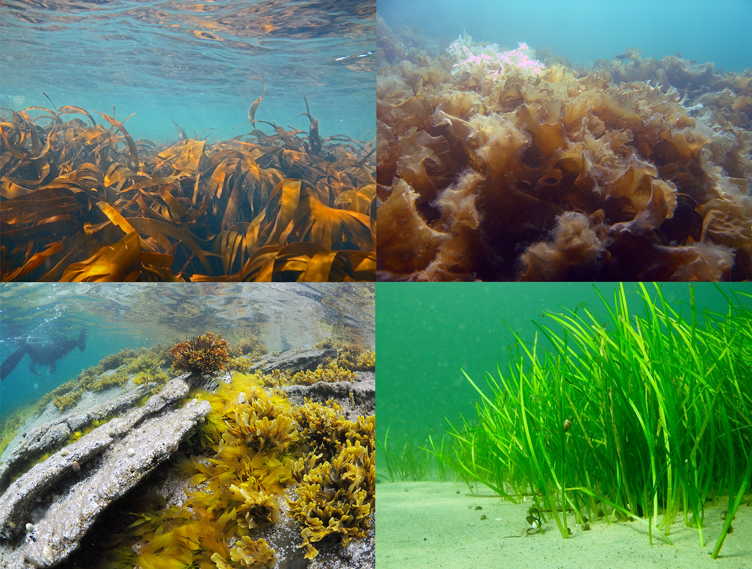
Figure 1. Photo examples of species and habitat types in this study.
From upper left: Tangle kelp (Laminaria hyperborea, ©Janne K. Gitmark, NIVA), sugar kelp (Saccharina latissima, © Hartvig Christie, NIVA), bladder wrack (Fucus vesiculosus, © Janne K. Gitmark), and eelgrass (Zostera marina, © Christoffer Boström).
Among the Nordic countries, kelp is most widespread along the rocky shores of Norway, Svalbard, Greenland, the Faroe Islands, Iceland and Sweden´s west coast. The rest of Sweden has few kelp forests due to the low salinity of the Baltic Sea, while Finland has no kelp forests at all. Denmark's coastal areas are mostly covered by soft sediments suitable for seagrass, whereas rockweed, kelp and other attached algae are confined to scattered stones and a few stone reefs. In Norway, rockweed and seagrass make up a relatively small proportion of blue forest areas (Gundersen et al., 2011) compared to kelp, whereas in the Baltic Sea, rockweed dominates.
Methods
Distribution models for the two kelp species, tangle kelp (Laminaria hyperborea) and sugar kelp (Saccharina latissima) were individually developed for Norway since there are high-resolution environmental maps available for Norway, but not for the whole of the Nordic region. Kelp distribution models for the Nordic region were subsequently developed using a compiled dataset covering most of the Nordic countries. Norwegian rockweed was analyzed using a simple rule-based GIS model, while Swedish seagrass and Danish and Swedish rockweed were extrapolated from known distributions from parts of the coastline. The remaining distribution estimates for seagrass and rockweed were retrieved from existing literature and databases. For Greenland and the Faroe Islands, no data were available for the mapping of large scale distribution of rockweed and seagrass.
The Norwegian kelp dataset
For Norway, the data were mostly sampled through the Norwegian Program for Mapping Biodiversity (Bekkby et al., 2013). The program is designed for tangle kelp (n = 11 891 observations) primarily, but also sugar kelp data (n = 11 053) are registered when found. Thus, the Norwegian dataset is suitable for modelling tangle kelp, but less suitable for sugar kelp. Data are registered using an underwater video camera with an approximate observation window of “a few square meters”. Density categories are quantified as absence, single plants, scarce, moderately dense, and dense forest, representing density categories of 0, 0.1, 0.5, 5 and 10 individual kelp plants per m2 for tangle kelp and 0, 0.5, 1, 7 and 15 for sugar kelp, which usually has a higher number of plants per m2 than tangle kelp. “Individual plants per m2” was thus the unit used in the statistical analyses, with the benefit that densities of kelp were predicted directly, which is a more quantitative measure than the probability of kelp forest presence.
The Nordic kelp dataset
The data used in the Nordic kelp distribution model were compiled from several sources, and sampled using somewhat different methods and measures for kelp quantities. The datasets were therefore challenging to combine to a unified dataset for the Nordic analyses. The solution was to convert all measures to presence/absence of kelp forest and setting cut-off values based on expert judgement of what would be considered as a kelp forest as compared to less dense kelp areas. Observations of high-densities (plants per m2) or high coverage would then be presence, and low coverage, including observations of other species than those in focus, and would then be used as absence data in the analyses.
The Swedish dataset is owned by the Swedish Meteorological and Hydrological Institute (SMHI), provided by Susanne Baden at the University of Gothenburg. The dataset consisted of many different species of kelp, rockweed and seagrass, whereas only tangle kelp and sugar kelp were used for the statistical modelling. Note that “tangle kelp” includes here observations of both Laminaria hyperborea and the ecologically similar oarweed (Laminaria digitata). The data were given as two different quantitative measures: density (kelp plants per m2) and % coverage of the seafloor. As the % coverage data encompassed a larger area, only these data were used for the analyses, after being converted to presence/absence using a cut-off of 50% coverage to be defined as a kelp forest (n = 6 966 for tangle kelp and n = 7 049 for sugar kelp).
The Danish kelp dataset, originating from the Danish marine monitoring programme, was provided by Jacob Carstensen at Aarhus University and consisted of 221 species of macroalgae and others, including tangle kelp (n = 6 633, as for Sweden including both L. hyperborea and L. digitata) and sugar kelp (n = 6 526). The quantitative measure of kelp was given as % coverage, and also here 50% coverage was decided as the cut-off value for kelp forest. As most of the Danish coast is soft bottom, it is not suited as a macroalgae habitat. However, there is still some growth of kelp in this region, at localities with occurrences of scattered stones or genuine stone reefs.
The Greenland dataset consisted of underwater video transect data from the west coast, with records of different kelp species. The transects were georeferenced at each start and end point, but not along the transect line. We therefore set all locations along the transect to the start coordinates. Nevertheless, depth could still be included as a predictor variable in the analyses because the predictor layers in the Nordic model were of such low resolution (~1 km) that the whole transects (a few 100 m) were covered by one single grid cell and thus had an equal environmental profile. The two types of sugar kelp (S. latissima and S. longicruris) (n = 788) were modelled together in our analyses, since they are assumed to respond similarly to environmental variables (Neiva et al., 2018). Tangle kelp is not reported from Greenland and was set as absences in the locations of the transects. There is also some recent data sampled by Susse Wegerberg and Ole Geertz-Hansen (Aarhus University) from the east and south coast of Greenland, but this had not been quality checked at the time of writing and could not be included in the Greenland dataset.
A comprehensive dataset from the Finnish Inventory Programme for the Underwater Marine Environment (VELMU) was provided by Christoffer Boström from Åbo Akademi University. This dataset consisted only of different species of rockweed and seagrass. The lack of kelp in this dataset is expected, since the Baltic Sea is not within the natural distribution range of kelp. The Finnish dataset could however be used as confirmed absences for the Nordic presence/absence models. A random sample of 25% (n = 4 266) was used to avoid slowing down the model run too much.
A small (n = 298), but very appreciated dataset from the Faroe Islands was provided by Grethe Bruntse (formerly of Kaldbak Marine Biological Laboratory) from the FARCOS project. Tangle kelp (grouped with other Laminaria species) and other macroalgae were quantified according to a 7-level coverage scale as > 90%, 50–90%, 20–50%, 5–20%, < 5%, single plants or scarcer. A cut-off value was set at 50% coverage for kelp forest.
Although we are aware that the Marine and Freshwater Research Institute holds some distribution data from the coast of Iceland, we were unable to obtain this for inclusion in our analyses. The predictions made for Iceland are therefore extrapolated from the general Nordic model.
Data for Norway were also incorporated into the Nordic model, using the same dataset as in the Norwegian model described above. For the Nordic model, where we focused on the presence of kelp forest instead of densities of individual plants, we defined presence as ≥5 plants per m2 for tangle kelp and ≥7 for sugar kelp. The two kelp datasets were mostly sampled from the same stations, thus a presence of one species is then used as an absence of the other.
Environmental variables used in the analyses
In fitting the models for Norway, we used field-measured depth and a range of environmental variables extracted from both national and global spatial datasets. Wave exposure (km2/second) was extracted from a model with a 25 m spatial resolution (Isæus, 2004) based on fetch, wind speed and wind frequency. Ocean current speed (m/s) was modeled at a horizontal resolution of 800 m (NorKyst-800; Albretsen et al., 2011) using the three-dimensional numerical ocean model ROMS (Shchepetkin & McWilliams, 2005; Haidvogel et al., 2008) and downscaled to 25 m resolution. The 90th percentiles (i.e., the 10% highest values) for seabed currents were used in our analyses. Due to the lack of a full cover, high resolution substrate model, which does not exist for Norway, slope (°) and terrain curvature (m) were derived from a bathymetry model with a 25 m horizontal resolution, provided by the Norwegian Hydrographic Service. Terrain curvature was estimated with a 250, 500 and 1 000 m spatial calculation window (Bekkby et al., 2009). These two variables were used as proxies for substrate under the assumption that gentle slopes and depressions are areas of higher likelihood of sedimentation and thus not hard substrate. Light at the seabed (photosynthetically active radiation, PAR) has been modeled using data from ocean color satellite sensor estimates (Saulquin et al., 2013, Populus et al., 2017) at a resolution of 100 m. Light at the seabed was downscaled to a model with 25 m resolution. All predictor variables given above, including the 25 m bathymetry model, were available as full cover GIS layers and used for making predictive distribution maps for kelp.
We also included variables from the global Bio-ORACLE datasets on temperature and salinity at mean, maximum and minimum depths (within grid cells of 5 arc-minutes resolution, which corresponds to slightly less than 10 km at the equator). Even though the resolution is relatively low, we chose to use Bio-ORACLE for temperature and salinity data in the hope of utilizing their future climate projection layers for these variables (corresponding to predictions for the different RCP scenarios). It will eventually be possible to plug these predictions into the model to make scenarios for future kelp distribution, plant densities and biomass along the Norwegian coast.
Similarly, separate distribution models for tangle kelp and sugar kelp were fitted for the full Nordic region using the combined presence/absence data. As environmental variables, we extracted photosynthetically available radiation (PAR, mean and max) and current velocity (mean and range) from Bio-ORACLE. Furthermore, we included data on east/west aspect, north/south aspect, distance to shore, bathymetric slope, sea surface salinity (mean and range), sea surface temperature (mean, range, max and min) and sea ice concentration (mean) from the global ocean climate layers MARSPEC, which were available at a higher resolution than Bio-ORACLE (30 arc-seconds resolution, which equals ~1 km at the equator). We also included wave fetch data from a 100 m European GIS layer available from Burrows (2020), that unfortunately did not cover Greenland. Similarly, substrate data were only available for some locations around Scandinavia (EMODnet’s 5 category layer). For other areas, these variables were set as missing. For bottom depth, we used field measurements.
Statistical models
Boosted regression tree (BRT) models for the spatial distribution of kelp densities (tangle kelp and sugar kelp, separately) on the Norwegian and Nordic levels were built using the gbm (Greenwell et al., 2019) and dismo (Hijmans et al., 2017) libraries in the statistical program R. BRT models have several advantages over traditional regression techniques such as Generalized Linear Models (GLMs) or Generalized Additive Models (GAMs). For example, a large number of predictor variables of different types (e.g. interval and class) can easily be implemented without prior data transformation; potential interactions between variables are automatically handled; and missing values are accommodated. We performed preliminary analyses which compared BRT models with GAMs and found that the BRT models performed better for both kelp species and at both the Norwegian and Nordic level.
For Norway, the response variable was kelp density, i.e. the number of plants found per square meter. All environmental GIS layers were resampled to a resolution of 25 m before predictions were made. Both models therefore have a resolution of 25 m, but it is important to keep in mind that some of the underlying information is of a lower resolution.
For the Nordic region, BRT models were built with presence/absence of kelp forest as a response variable. Here too were tangle kelp and sugar kelp modelled separately, however, note that observations of L. digitata were included with L. hyperborea in the tangle kelp model, and S. longicruris with S. latissima in the sugar kelp model. All environmental GIS layers were resampled to a resolution of 30 arc-seconds (~1 km) for predictions, using bathymetry data from MARSPEC to cover the full region. Based on these models, we predicted the probability of presence of kelp forest across the Nordic region. All environmental GIS layers were resampled to a resolution of 30 arc-seconds (~1 km) for predictions, using bathymetry data from MARSPEC to cover the full region.
Estimating kelp area
The Norwegian and the Nordic models resulted in full cover maps predicting the densities (individual kelp plants per m2) and the probability of kelp forest, respectively. To be able to estimate the kelp forest distribution area at the Nordic level, we converted each grid cell in the Nordic prediction map to predicted presence or absence of kelp forest. This was done using the threshold function in the dismo library in R to set a cut-off value for separating forest from no forest, giving equal weight to sensitivity (true positive rate) and specificity (true negative rate).
To calculate the total predicted extent of kelp forest for Norway we first counted the number of grid cells with predicted ≥ 1 plant per m2 and then multiplied the answer with the area of each grid cell (625 m2). Area was also calculated for each density class (integers ≥ 1) to illustrate the distribution of kelp densities. Due to the lack of standard deviations provided by the BRT model, ranges for the Norwegian area estimates were set as the total area covered by densities ≥ 6 (minimum) and densities ≥ 4 (maximum), which were regarded as broad boundaries. For the Nordic models, which were given as probabilities rather than densities, we 1) calculated the area per grid cell (which is not a constant number since arc-minutes varies with latitude), 2) summed the area with predicted kelp forest according to grid cell size, and 3) split the total area by country using a shape file of the Nordic country’s Exclusive Economic Zones (EEZ), using the raster library in R. The potential range of areas was estimated as follows: for lower ranges, we calculated the models’ false positive prediction rates (predicted kelp forest in locations with absence in the data), multiplied these false positive rates with the estimated areas per country, and subtracted these “potentially overestimated areas” from the original estimates. For upper ranges, we calculated the models’ false negative prediction rates (predicted absence in locations with forest in the data), multiplied these negative prediction rates with the total areas of the countries’ EEZ that were not predicted to be covered by kelp forest and that were < 30 m bottom depth (based on the response to bottom depth in the models), and added these “potentially underestimated areas” to the original estimates.
The predicted distribution maps were then adjusted for two areas, after being scrutinized by Norwegian and Danish/Greenland kelp experts. First, we removed predicted kelp forest areas north of known kelp observations in Greenland, specifically, north of 74° 19′ N on the east coast and north of 77° 47′ N on the west coast (Dorte Krause-Jensen, personal observation). The rationale for this is a lack of ground truth data for the northern and eastern coasts of Greenland where extensive ice cover furthermore reduces the likelihood of abundant kelp forests. Secondly, we removed predicted kelp forest in areas of soft sediments in Denmark. The coast around Denmark is mostly soft bottom, with occasional stone reefs where kelp can grow. The overprediction of kelp in these areas was due to the coarse resolution of environmental layers, and thus masks the effects of variables with a high local variation, such as substrate type. The masking was carried out according to a detailed substrate layer available for Denmark from the Geological Survey of Denmark and Greenland.
Estimating the production from Norwegian kelp
The annual primary production from Norwegian tangle kelp is 42 (range 20–60) g carbon per plant per year, estimated using individual plant production derived from area-specific production in Pedersen et al. (2012, 2019) and Sjøtun et al. (1995). In the absence of similar production estimates from sugar kelp, we assumed the same production per m2 as for tangle kelp, resulting in 22 (range 10–32) g carbon per plant per year after adjusting for plant density. The total production for each kelp species was then estimated as density (number of kelp plants per m2) multiplied with the production (g carbon per individual), summed for all grid cells and finally multiplied with grid size (625 m2). See Chapter 3 for further calculations of kelp production.
Estimating the living biomass of Nordic kelp
To estimate the total living biomass of Norwegian tangle kelp, 14.4 kg per m2 was calculated from an available depth-specific biomass model (average from upper 10 m, Gundersen et al., submitted) and multiplied with the total kelp forest area (densities ≥5).
In the absence of a similar number for Norwegian sugar kelp, and kelp in general for the Nordic region, we assumed the same number (14.4 kg biomass per m2).
Seagrass distribution and living biomass
For Nordic seagrass distribution and living biomass estimates, we used already published literature and available databases. In the Nordic countries, monitoring and mapping have both been a lot more intensive for seagrass than for kelp and rockweed. Seagrass in Norway has been mapped through the Norwegian Program for Mapping Biodiversity (Bekkby et al., 2013), which ended in 2019 and is available at NEA’s database for nature types (naturbase.no). Along the Baltic Sea gradient, eelgrass occur in monospecific stands in the south but form multispecies meadows (mixed with freshwater plants) in the brackish northern parts. Seagrass meadows in this region have been thoroughly studied and mapped and are summarized in Boström et al. (2014), where estimates of coverage also are presented. However, since this study gives distribution estimates for sea regions rather than countries, these estimates could not be used directly in this study. For Denmark, a more recent estimate of potential eelgrass area coverage is given by Staehr et al. (2019), and for Finland, estimates based on the model published by Virtanen et al. (2018) were provided by C. Boström. For the Swedish west coast down to Øresund, Moksnes et al. (2016) estimated 197 km2 of seagrass. The total distribution of seagrass in Sweden was estimated by expert judgement (Per Moksnes, personal communication) based on this known part of the coastline. Also, the HELCOM metadata catalogue provides maps of seagrass for the Baltic region, but these estimates seem to be greatly overestimated, presumably because single point observations have been scaled up to coarse resolution maps. Our conclusion is that HELCOM data cannot be used for area estimates, only as areas of potential presence of the species. Also, for Denmark, the observations underlying the HELCOM polygons represent the historic data and are not representative of the present situation (Staehr et al., 2019). For Iceland, some relatively crude estimates were available from the Icelandic Institute of Natural History (IINH) website. Boström et al. (2014) also report Iceland seagrass distribution of approximately the same size, presumably based on the same data. In Greenland, there are known occurrences of eelgrass meadows in inner parts of protected fjord branches in the Nuuk fjord system and further south on Greenland’s west coast. These relatively small Greenland meadows have just as high biomass but slower biomass turn-over (production) as eelgrass elsewhere in the distribution range (Olesen et al., 2015; Clausen et al., 2014). Unfortunately, no data were available for seagrass area in the Faroe Islands.
To get estimates of living seagrass biomass on a national level for the Nordic countries, we multiplied the total distribution areas by 79 g C DW m-2, which is an average of the above ground carbon biomass stocks for the Baltic sea given by Röhr et al. (2018), and further converted them to living biomass using a factor of 0.38 (Atkinson and Smith, 1983) and 0.17 from DW to FW (Wickham et al., 2019b; Kraemer and Alberte, 1993; J. Thormar, unpubl. data). We are aware that this is a very rough simplification, since seagrass meadows vary considerably in terms of density, height, etc. Thus the estimates of living seagrass biomass should be interpreted with caution.
Rockweed distribution and biomass
In the absence of rockweed data in Norway, the distribution of this habitat type has previously been estimated by Gundersen et al. (2011) at 178 km2, using simple rule-based GIS models. There are still no data for Norway, but a somewhat more sophisticated rule-based model was drawn up in this study in order to make a more reliable estimate of the total rockweed distribution in Norway. All coastal areas between 2 m depth and 2 m above the coastline, assumed to represent the littoral zone, were selected in a GIS using a 25 m bathymetry model. Knowing that approximately only 56% of the Norwegian coast is rocky shore (Young & Carilli, 2018), this fraction was multiplied with the estimated area to exclude parts of the coastline assumed to be soft sediments. For the Baltic countries (Denmark, Sweden and Finland), rockweed (Fucus spp.) distribution data was available from the HELCOM metadata catalogue, but seagrass were assumed to be largely overestimated and therefore not used. Instead we used estimates based on models from Virtanen et al. (2018) for Finland. For Denmark and Sweden, we used the newly released area estimates of rockweed (Fucus) for Danish Kattegat given in Riemann (2020). These were extrapolated for the whole of Denmark and Sweden assuming the same amount of rockweed per kilometer for the whole coastline, excluding areas with known low distributions, which were the Danish west coast and the northern east coast of Sweden. For Iceland, estimates of rockweed were available from the IINH website. As for seagrass, no rockweed data was available for the Faroe Islands. We had no distribution estimate for rockweeds in Greenland, although rockweeds are abundant and can reach living biomasses exceeding 30 kg m-2 (e.g. Høgslund et al., 2014; Ørberg et al., 2018). Data on intertidal community cover and biomass, including rockweeds, have been compiled from south to north along Greenland’s west coast (Thyrring et al., submitted).
As for the seagrass, the rockweed areas were multiplied with a constant average weight and summed up to get living biomass estimates on the level of Nordic countries. The biomass estimate used for rockweed was 5 714 g per m2 based on Attard et al. (2018), after converting from C to biomass by a factor of 0.35 (Attard et al., 2018) and DW to FW using the same estimate as for kelp at 0.15 (Pedersen et al., 2019).
Results and discussion
Geographical distribution of Norwegian kelp
The distribution of the two kelp species sugar kelp (Saccharina latissima) and tangle kelp (Laminaria hyperborea) along the Norwegian coast was modelled separately. As mentioned earlier, the Norwegian kelp data predominantly stem from surveys conducted to document the distribution of tangle kelp, and data from typical sugar kelp areas are therefore underrepresented. This may also lead to observations of sugar kelp being biased towards low density registrations, and can contribute to an underestimation of densities, but not necessarily of the total distribution area. The tangle kelp model performed reasonably well, with a total deviance explained as close to 75% (a measure of variation in the data explained by the model) and correlation values between data and model predictions at 0.87 (based on training data) and 0.77 (based on cross-validation, CV). The sugar kelp model performed less well. Although the total deviance explained was approximately the same, the correlation values were much lower (0.84 and 0.62 for training data and CV, respectively) (Figure 42, Appendix A). We know from earlier studies that tangle kelp forests generally occupy wave exposed areas, while sugar kelp is found in more sheltered areas. Our models capture this pattern, as illustrated in prediction maps for the southern Møre region on the west coast (Figure 2 and Figure 3). The most important explanatory variables for tangle kelp were bottom depth, wave exposure and mean temperature (Figure 43, Appendix A), while for sugar kelp, the most important explanatory variables included bottom depth, longitude, maximum salinity and latitude (Figure 44, Appendix A). The importance of longitude and latitude reflects how spatial variation exists that the given set of variables did not account for. In the absence of a suitable substrate model for Norway, we used slope and terrain as proxies, as these variables affect the sedimentation rate and thus the substrate of the seafloor. However, even though we know substrate is an important driver of kelp forest distribution, slope did not come out as important in either model. Nevertheless, terrain curvature estimated with a 1 000 m spatial calculation window explained 12% of the total deviance in the sugar kelp model, while for tangle kelp, the three curvature variables (estimated with 1 000, 500 and 250 m calculation window) explained around 3–4% each.
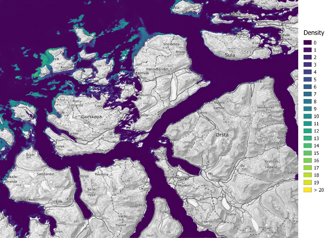
Figure 2. Tangle kelp (Laminaria hyperborea) densities (number of plants per m2), predicted for Norway based on field data and statistical analyses (Boosted Regression Tree modelling, BRT). The model is illustrated for the southern Møre region on the west coast of Norway, and has a spatial resolution of 25 m.
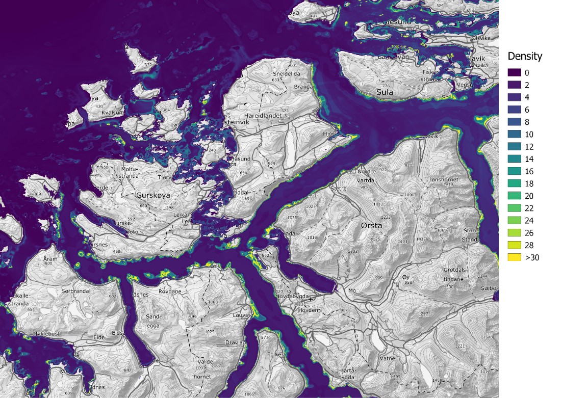
Figure 3. Sugar kelp (Saccharina latissima) densities (number of plants per m2), predicted for Norway based on field data and statistical analyses (Boosted Regression Tree modelling, BRT). The model is illustrated for the southern Møre region on the west coast of Norway and has a spatial resolution of 25 m.
Predicted areas of Norwegian kelp forests
When including all areas with densities ≥1 plant per m2, we estimated the total area covered by tangle kelp to be 18 155 km2, and 44 300 km2 for sugar kelp. However, when including only high-density areas, by setting cut-off values for forest at ≥5 for tangle kelp and ≥7 for sugar kelp, these numbers were reduced to 3 810 km2 and 3 607 km2. These numbers are slightly lower for tangle kelp and higher for sugar kelp compared to former estimates by Gundersen et al. (2011), who estimated 5 900 km2 and 2 000 km2 for tangle kelp and sugar kelp, respectively, using a rule-based GIS model. It should also be taken into consideration that, since Gundersen et al. (2011) made these estimates, there has been a significant regrowth of kelp (mostly sugar kelp) following sea urchin destruction.
The new kelp distribution models provided very detailed maps of densities, which varied greatly depending on environmental factors (Figure 2 and Figure 3). Insight into this spatial variation showed that there are vast areas with low densities of kelp forest along the Norwegian coast, compared to the high-density forests (Figure 4). The primary production is calculated and presented in Chapter 3.
Figure 4. Predicted size (km2) of kelp areas, for tangle kelp (Laminaria hyperborea, upper two panels) and sugar kelp (Saccharina latissima, lower two panels), shown as total area (for each density class, left two panels) and accumulated according to the different density thresholds (right two panels).
Geographical distribution of kelp forests in the Nordic countries
For the Nordic region, tangle kelp (including Laminaria digitata) and sugar kelp (including Saccharina longicruris) were modelled separately as presence/absence of forests. The tangle kelp model again performed better than the sugar kelp model, with a total deviance explained of 67% vs. 54%, and correlation values between data and model predictions of 0.82 vs. 0.67 (based on training data) or 0.78 vs. 0.58 (based on cross-validation, CV), respectively (Figure 45, Appendix A). This may relate to issues with the Norwegian data as explained above, or patterns in the data from other countries. The most important explanatory variables for tangle kelp distribution were minimum sea surface temperature, bottom depth and wave fetch (Figure 46, Appendix A), while for sugar kelp, bottom depth was clearly the most important variable, with several other variables, including sea surface salinity range and east-west aspect, playing a lesser role (Figure 47, Figure 45, Appendix A).
Despite the coarser resolution of the Nordic models (approximately 1 km), the models captured the different affinities of tangle kelp and sugar kelp to exposed and sheltered areas, respectively, as illustrated when comparing predictions for the southern Møre region from the high-resolution Norwegian models (Figure 2 and Figure 3) with the Nordic models (Figure 5 and Figure 6).
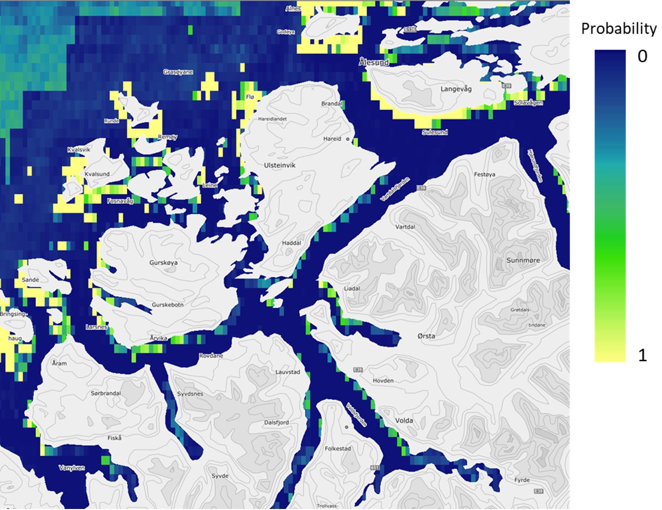
Figure 5. Predicted probability of occurrence of tangle kelp forests (Laminaria hyperborea) in the Nordic countries, based on field data and statistical analyses (Boosted Regression Tree modelling, BRT). The model is illustrated for the southern Møre region on the west coast of Norway and has a spatial distribution of approximately 1 km. The probabilities shown here were converted to presence/absence of forest in the final prediction maps (Figure 7).
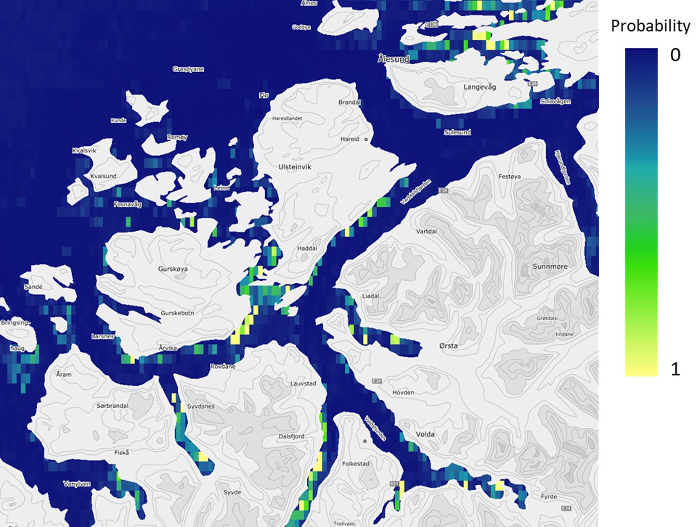
Figure 6. Predicted probability of occurrence of sugar kelp forests (Saccharina latissima) in the Nordic countries, based on field data and statistical analyses (Boosted Regression Tree modelling, BRT). The model is illustrated for the southern Møre region on the west coast of Norway and has a spatial distribution of approximately 1 km. The probabilities shown here were converted to presence/absence of forest in the final prediction maps (Figure 7).
Overall, the Nordic models indicated that tangle kelp forests are found along the Norwegian coast and the northwestern Swedish coast, on the western coast of Denmark and in some locations in Kattegat, around the Faroe Islands, and on the southern coast of Iceland (Figure 7). The distribution of data input to the models is shown in Appendix A (Figure 48). For sugar kelp, the model predicted presence of forest along the Norwegian coast northwards to Lofoten, along the western Swedish coast, in some areas in the Kattegat, and on the western coast of Denmark (Figure 7). Because of the coarseness of the substrate layer, the model greatly overestimated kelp forest distribution in Denmark. Therefore, we removed the predicted kelp forest in Danish soft bottom areas from the map (see methods). The resulting kelp forest maps and area estimates for the Nordic countries (excluding Greenland) are shown in Figure 7 and Table 1. The model also predicted presence of sugar kelp all along the coast of Greenland, including the north coast, which is known to be seasonally or permanently covered with ice, which means that presence of kelp forests there is therefore unlikely. This overestimation is most likely due to limited data on the absence of kelp for northern Greenland, and predictions were therefore removed from the map in northern Greenland (see methods). Prediction maps for Greenland sugar kelp are shown in a separate map (Figure 49, Appendix A).
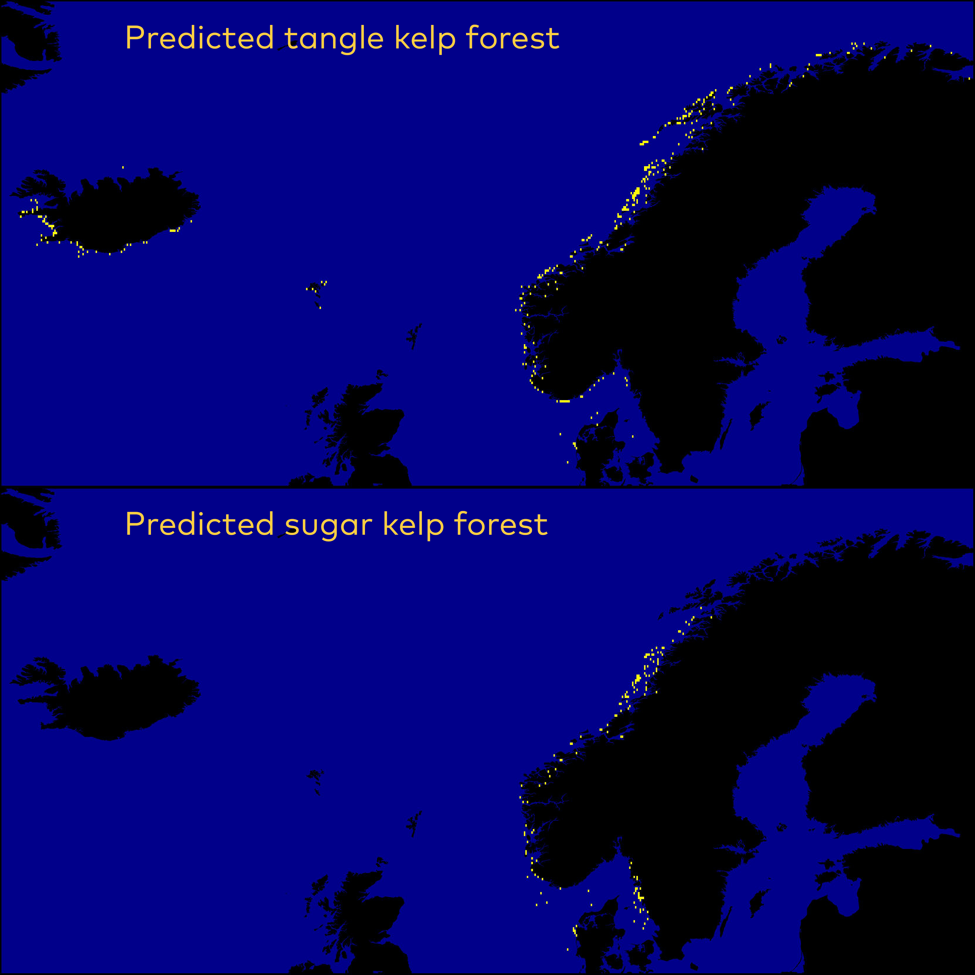
Figure 7. Predicted presence (yellow points) of tangle kelp (Laminaria hyperborea or L. digitata, upper) and sugar kelp (Saccharina latissima or S. longicruris, lower) forests across the Nordic region. The modelled presence is based on the probability models illustrated in Figure 5 and Figure 6, and has a spatial resolution (grid cell size) of approximately 1 km.
Predicted areas of Nordic kelp forests
The predicted areas covered by tangle kelp and sugar kelp forests within each Nordic country’s Exclusive Economic Zone (EEZ) are given in Table 1. The predicted area of tangle kelp forests exceeded sugar kelp in Norway, as also found in the Norwegian model. The differences between the Nordic and the Norwegian models for Norway might be due to the coarser spatial resolution of the Nordic model resulting in higher estimated habitat of tangle kelp, while for sugar kelp, the Norwegian model includes large areas with few kelp plants that are excluded in the Nordic model of presence/absence of kelp forest. In Sweden, the model predicted larger areas of sugar kelp than tangle kelp, likely because most of this coastline is relatively sheltered, while in Finland, neither species was predicted to be present (as shown in the data, Figure 43 in Appendix A). As discussed above, the original predicted distributions for Denmark were clearly overestimated, as much of the Danish coast is covered by soft bottom not suitable for kelp. We therefore decided to remove Denmark from the area estimates for the Nordic region. For the Faroe Islands, tangle kelp is predicted to cover larger areas than sugar kelp, as indicated by tangle kelp (Laminaria digitata) being more common than sugar kelp in the Faroese dataset. For Greenland, the model clearly reflects the absence of tangle kelp in the data. For sugar kelp, we masked any predictions north of known observations of kelp, and the total area was estimated to be 26 704 km2.
| Country | Tangle kelp (km2) | Sugar kelp (km2) |
| Norway (25 m) | 3 810 (2 934-4 925) | 3 607 (2 999-4 392) |
| Norway | 9 342 (8 719-10 775) | 4 435 (4 068-4 916) |
| Sweden | 127 (119-1 148) | 858 (785-1 180) |
| Finland | 0 (0-787) | 0 (0-251) |
| Denmark | NA | NA |
| Faroe Islands | 235 (219-263) | 10 (9-20) |
| Iceland | 2 328 (2 173-2 774) | 15 (14-168) |
| Greenland | 2 (2-3 823) | 26 704 (24 491-27 877) |
| Total | 6 502 (5 447-13 720) | 31 194 (28 298-33 888) |
| Total | 12 034 (11 232-19 570) | 32 022 (29 367-34 412) |
Table 1. Predicted size (km2) and ranges (min-max) of tangle kelp (Laminaria hyperborea or L. digitata) and sugar kelp forests (Saccharina latissima or S. longicruris) across the Nordic region, as modelled in the present study and illustrated in Figure 7. Estimates from the more detailed (higher spatial resolution) Norwegian 25 m resolution model are included in a separate row for comparison purposes, as they are regarded as more reliable than those from the Nordic model. Estimates for Norway from the Nordic model are shown in light grey for the same reason.
Area estimates of Nordic seagrass
The total distribution of seagrass meadows in Norway has been estimated at 60 km2 through the Norwegian Program for Mapping Biodiversity (downloaded from naturbase.no). This can be regarded as a conservative estimate, since only confirmed meadows are included. Following the rationale used in the Norwegian red list of species, this area was multiplied by a factor of 1.5 to include meadows assumed to be present but not recorded (Table 2). The HELCOM metadata catalogue was visited to obtain estimates on seagrass for Sweden (4 640 km2), Finland (1 816 km2) and Denmark (6 700 km2), but since they were assumed to be overestimated (see methods), they were not used in this study. For Denmark, the estimate from Staehr et al. (2019) of 2 204 km2 was used as a more reliable and up-to-date estimate on potential seagrass distribution. For Finland, the model published by Virtanen et al. (2018) estimated 6 km2 in total. The total distribution of seagrass in Sweden was estimated at ca. 300 km2 (range 200–400) by expert judgement (Per Moksnes, personal communication). The Icelandic seagrass area estimate was retrieved from the IINH website. Since this information was only in Icelandic, we lack information on how these estimates were arrived at and whether they can be assumed to be realistic, overestimated or underestimated. No data on seagrass distribution has been available for the Faroe Islands or Greenland (see methods), however, the ongoing CARMA project (2018–2021), with the aim of exploring the role of Arctic kelp forests in carbon sequestration, will likely also result in some estimates of seagrass for Greenland. Great interest surrounds the warming Arctic region, and we can expect some major changes of macroalgae distributions around Greenland as the ice melts and the ocean temperature rises.
Area estimates of Nordic rockweed
Norwegian rockweed area estimated in this study resulted in a total area of 3 090 km2. This is higher than presented earlier by Gundersen et al. (2011), but is assumed to be more realistic, due to slightly more sophisticated methods when using information on bathymetry instead of just a constant buffer of 1 meter around the coastline. The predicted seagrass sizes for Denmark and Sweden extrapolated from Rieman (2020) were 397 km2 and 1 335 km2, respectively. The Icelandic rockweed area estimate was retrieved from the IINH website. Due to limited data, no rockweed distribution area could be modelled for the Faroe Islands or Greenland, but updates on rockweed distribution from Greenland are expected in the ongoing CARMA project.
| Country | Seagrass (km2) | Rockweed (km2) |
| Norway | 90 (Naturbase) | 3 090 (This study) |
| Sweden | 300 (P. Moksnes personal communication) | 1 335 (This study) |
| Finland | 6 (Virtanen et al., 2018) | 239 (Virtanen et al., 2018) |
| Denmark | 2 204 (Staehr et al., 2019) | 397 (This study) |
| Faroe Islands | NA | NA |
| Iceland | 11 (IINH) | 495 (IINH) |
| Greenland | NA | NA |
| Sum | 2 611 | 5 556 |
Table 2. Predicted size (km2) of seagrass and rockweed areas across the Nordic country’s Exclusive Economic Zones (EEZ) based on data from existing literature and databases and models developed as part of this study (Norwegian, Swedish and Danish rockweed areas).
Biomass of blue forests in the Nordic countries
For tangle kelp, the standing stock (i.e. living biomass) was calculated using a newly developed depth-specific biomass model (Gundersen et al., submitted). The living biomass of tangle kelp for Norway was estimated at 55 million tonnes. The corresponding estimate for sugar kelp was 52 million tonnes of biomass based on certain assumptions of similarities with tangle kelp. The total Nordic living biomass of kelp was 158 million tonnes, divided into 93.6 (59%) and 64.7 (41%) for tangle kelp and sugar kelp, respectively. Greenland was excluded from these estimates due to the largely uncertain area estimates.
Using estimates of aboveground standing biomass of eelgrass by Röhr et al. (2018) of 300 g C m-2 (Table 8), the total living biomass of seagrass in the Nordic countries was 3.2 million tonnes (2 611 km2 x 1.23 kg m-2). Using estimates of carbon stocks in living biomass of rockweed by Attard et al. (2018), the total living biomass of rockweed in the Nordic countries was 31.8 million tonnes (5 556 km2 x 5.71 kg m-2).
Conclusions
In this chapter, we estimated the distribution and biomass of blue forests in Norway and the Nordic region. Using novel high-resolution prediction models, we found that the total area where kelp is present in Norway was as much as 18 000 km2 for tangle kelp (Laminaria hyperborea) and 44 000 km2 for sugar kelp (Saccharina latissima). However, when including only high-density areas with more than 50% coverage of kelp plants, the kelp areas are reduced to 3 800 km2 and 3 600 km2, respectively. These estimates are not drastically changed from earlier estimates by Gundersen et al. (2011), which were 5 900 km2 and 2 000 km2 for tangle kelp and sugar kelp and based on less sophisticated methods, but still worth noting the differences, for instance regarding the harvesting of tangle kelp. The new maps provide more detailed information on how the density of kelp varies with depth, exposure and other environmental variables. A newly developed depth-specific kelp biomass model from NIVA was used to translate the distribution estimates to a total of 107 million tonnes of living kelp biomass for Norway. Summed at the Nordic level (Greenland excluded), we estimated approximately 6 500 km2 and 5 000 km2 of tangle kelp and sugar kelp forest, respectively.
Based on existing literature and available databases, the Nordic seagrass meadows cover 2 600 km2. This estimate does not include the Faroe Islands and Greenland, due to lack of distribution estimates, although there are known occurrences of high-density seagrass meadows on Greenland’s west coast. The total Nordic area of rockweed summed up to 5 550 km2, excluding Greenland and the Faroe Islands.
The total living biomass of kelp in the Nordic countries is estimated at 158 million tonnes (Greenland excluded). The living biomass of seagrass and rockweed amounted to 3.2 tonnes and 31.8 million tonnes, respectively (excluding Greenland). A crude procedure was used to convert area estimates to these measures of living biomass. In the knowledge that there is a huge variation in biomass based on the environmental factors throughout the Nordic regions, the lack of spatial models of biomass forced us to use single estimates for each habitat type to be multiplied with area estimates in order to measure the living biomass for the Nordic region. The estimated living biomass should therefore be used with caution.
The estimates of distribution and biomass are based on several assumptions and simplifications, but still represent the first pan-Nordic overview of blue forest habitats. Key uncertainties are to a large extent related to the distribution of kelp in Greenland and Denmark, and highlight the need for high-resolution data input on depth and substrate to improve prediction maps, as well as data for kelp for larger parts of the Nordic region, such as Greenland and the Faroe Islands, and rockweed for most of the Nordic region. Seagrass is studied thoroughly in the Baltic region and is also mapped for Norway, but there are large data gaps for Greenland and the Faroe Islands.
Chapter 2 – Field|work on kelp carbon ex|port and long-|term sto|rage of kelp carbon
Organic carbon produced by macroalgae is exported to and stored in coastal and deep-sea sediments and plays an important role in long-term carbon storage (termed carbon sequestration). This way, macroalgae including kelp forests have potential for climate change mitigation. Nevertheless, there are few studies on sedimentation rates, turnover and long-term storage of kelp carbon in marine sediments. The lack of empirical data makes today's estimates of turnover and sequestration rates of carbon highly uncertain (Duarte et al., 2005; Krause-Jensen & Duarte, 2016; Gundersen et al., 2011).
Parts of kelp plants are transported out of the kelp forests as detrital matter, due to blade erosion or detachment of entire plants. The carbon fraction of the kelp detrital matter is termed kelp particulate organic carbon (kelp POC). Kelp POC is thus exported out of the kelp forest and deposited in shelf or deep-sea sediments, where it is either turned over or buried in the sediment and potentially sequestered.
Another fraction of the carbon that is fixed during photosynthesis in kelp is released as dissolved organic carbon (DOC), termed kelp DOC. Export of kelp DOC represents another important component to the carbon export from macroalgae, but lack of data and large uncertainties in the DOC production and export mean that its contribution to the blue carbon budget and sequestration potential are extremely uncertain (Watanabe et al., 2020). Part of the exported DOC is consumed by microorganisms (mainly bacteria) and the carbon part is returned to the atmosphere as CO2. However, a refractive part (not available to the food web) is exported from the habitats and eventually transported below the mixed zone of the large oceans and can contribute to long-term storage of carbon in the deep sea (Krause-Jensen & Duarte, 2016).
The aim of this work package was to provide key values based on new empirical data for the Nordic blue carbon budget: 1) how much kelp POC is buried and stored long-term (sequestered) in Norwegian marine sediments and 2) how much kelp DOC is produced and exported from kelp forests. The values are part of an updated blue carbon budget and improve the estimation of the potential for long-term storage of kelp carbon in marine sediments and in the deep sea.
Sediment cores were sampled in Frohavet in Trøndelag (Mid-Norway), providing core profiles of sedimentation rates and total organic carbon content (TOC) down to approximately 50 cm sediment depth. A novel eDNA technique was developed to identify and quantify the fraction of kelp carbon in the sediments originating from tangle kelp (Laminara hyperborea) and sugar kelp (Saccharina latissima). Stable carbon and nitrogen isotopes were applied as support parameters to investigate differences between sediments in terms of sources of carbon (C) and nitrogen (N). In order to quantify the DOC production and export from kelp, DOC production was measured from living kelp individuals in an in situ (in the field) incubation experiment at Malangen fjord, Troms (Northern Norway).
Methods
Study area and sediment core sampling
Frohavet is the sea between the Fosen Peninsula and the island of Froan in Trøndelag, at the north-west coast of Norway (63–64°N). It borders the island Frøya in the southwest, Bjugn in the southeast and the municipality of Åfjord in the east. It is a highly dynamic coastal environment with high primary productivity coming from both benthic macroalgae (kelp and rockweed) and phytoplankton in the water column. The main basin covers around 1 300 km2, with depths ranging from 100 to 500 m.
The stations for sediment core sampling are aligned in a transect in a northeast to southwest direction (Figure 8 and Table 3). Station 34 is the northernmost station, followed by station 31 approximately 7.5 km to the southwest. These two are the deepest stations with water depths of > 500 m and located in depressions in the seafloor which are assumed to be places where organic matter accumulates. Station 36 is located northeast of the island Tarva and 14.6 km to the southwest of station 31. Station 38 is the southernmost station, located between Tarva and Frøya and 12 km southwest of station 36. Stations 36 and 38 are located in areas of flat sea bottom at 354 and 242 m depth, respectively. In total, 13 sediment cores were sampled during fieldwork. However, the project budget only allowed for four cores to be analyzed further (primarily due to costs for sediment age analysis (210Pb)).
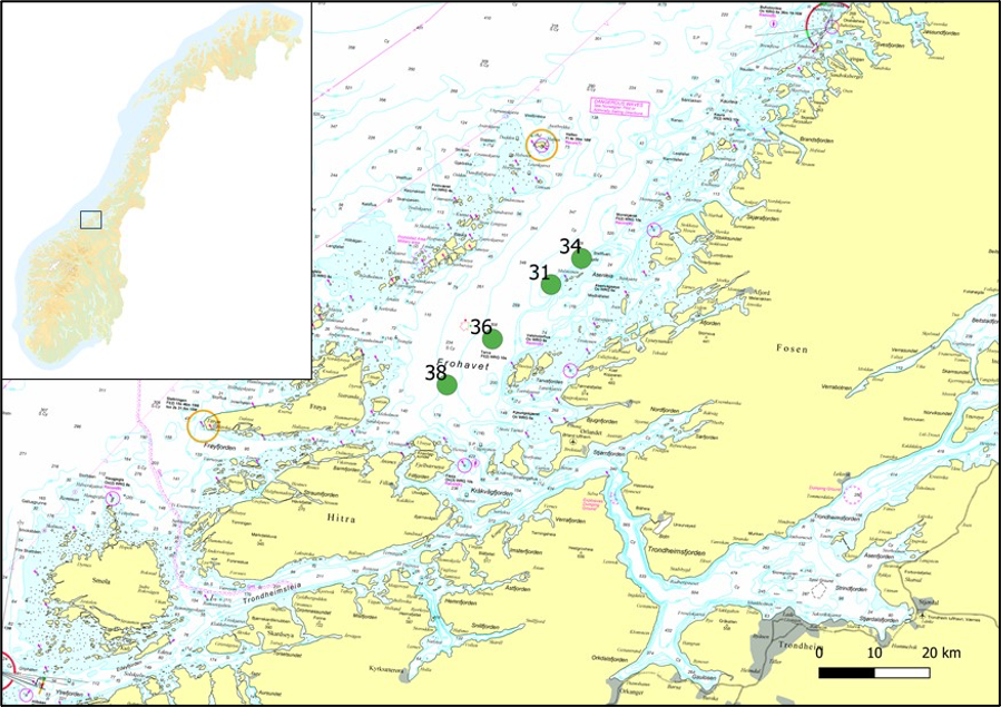
Figure 8. Map of the stations selected for sediment core sampling in Frohavet, Trøndelag (NW coast of Norway, 63–64°N). The selected stations represent a depth gradient from 242 m (#38) to 531 m (#31), see more details in Table 3.
| Station # | Date | Depth (m) | Lat | Long | Core length (cm) |
| 31 | 16.10.2018 | 531 | 63,9489 | 9,4852 | 100 |
| 34 | 16.10.2018 | 515 | 63,9953 | 9,5895 | 83 |
| 36 | 17.10.2018 | 354 | 63,8523 | 9,2878 | 61 |
| 38 | 17.10.2018 | 242 | 63,7715 | 9,1367 | 121 |
Table 3. Summary of the selected sediment core sampling stations in Frohavet, Trøndelag (NW coast of Norway, 63–64°N), including date of sampling, depth (m), geographical position (decimal degrees) and the length of each sediment core (cm).
Sediment core sampling was carried out in October 2018 from the NTNU research vessel R/V Gunnerus, with Captain Arve Knudsen at the helm. Sediments were sampled using a KC Denmark Gravity Corer (Figure 9). The corer recovers an 88.9 mm diameter and up to about 150 cm tall core of undisturbed sediment. A total of 13 sediment cores were collected, with core length ranging from 32 cm to 146 cm (Table 3). The sediment cores were capped with a bit of water from the sampling at the top and stored upright for transport to the laboratory where they were stored in the dark at 4°C until processing.

Figure 9. Sampling of sediment cores in Frohavet, Trøndelag (NW coast of Norway, 63–64°N) in October 2018 using a KC Denmark Gravity Corer. Photo: NIVA.
Sediment core processing
Sediment cores were processed in the laboratory and sliced into 1 cm thick sections, from the surface to 50 cm depth (Figure 10). From each core, 12 sections were chosen for further analysis: 0–1, 2–3, 4–5, 6–7, 8–9, 10–11, 13–14, 17–18, 22–23, 28–29, 35–36, 43–44 cm depth layers. Each section was analyzed for:
- Sediment age (210Pb)
- Total organic carbon (TOC) + total carbon (TC) content
- Chlorophyll a (Chl-a) content
- Genetics/kelp DNA abundance (quantitative PCR)
- 13C and 15N stable isotopes

Figure 10. Processing of a sediment core in NIVAs laboratory. Photo: NIVA.
Sediment dating (210 Pb)
The 210Pb dating technique was used to determine the chronology of each core and to estimate the sediment age of the different sediment layers. The method is accurate for sediment age up to approximately 120 years and will also provide sedimentation rates for each layer. The Department of Geosciences and Natural Resource Management at the University of Copenhagen carried out the 210Pb analysis and sediment dating. Sediment age for layers older than 120 years was extrapolated based on a function derived from a polynomial curve with R2 > 0.99.
Total organic carbon, total carbon and chlorophyll a content in the sediment cores
Total organic carbon (TOC) and total carbon (TC) content in the sediments was analyzed at NIVA’s laboratory using a CHN (i.e. carbon, hydrogen and nitrogen) elemental analyzer. TOC was quantified after removal of inorganic carbon by adding hydrochloric acid (HCl). Chlorophyll a pigments were extracted from the sediments by adding a defined volume of 96% ethanol, and concentrations were determined spectrophotometrically (Parsons & Strickland, 1963) using extinction coefficient as suggested by Wintermans & DeMots (1965). Chlorophyll a was analyzed at the Department of Biology at the Norwegian University of Science and Technology (NTNU).
Sediment grain size analysis
Sediment grain size distribution was determined by wet sieving through 2 000 µm, 1 000 µm, 250 µm, 125 µm, and 63 µm meshes, and calculated as a proportion of total sediment. Dry weight samples were classified according to the Wentworth scale (Wentworth, 1922). The grain size distributions were analyzed at Akvaplan-niva’s laboratory.
Species-specific qPCR assay development and core sample extraction
Among published kelp barcode sequences, the mitochondrial Cytochrome C Oxidase subunit I (COI) gene marker seemed to be the best choice - in terms of diversity among available sequences - for developing species-specific primers for the two targeted species. Sequences were aligned using CodonCode Aligner version 9.0 (CodonCode Corporation, MA, USA), and primers were developed using Oligo version 7.6 (Rychlik, 2007), resulting in two primer pairs for tangle kelp and three primer pairs for sugar kelp selected for testing. A BioRad CFX96 instrument was used to perform all quantitative polymerase chain reaction (qPCR) assay optimization and sample testing. The annealing temperature was determined by running gradient qPCR on both extracted species reference material and sediment cores. A primer pair producing an 88 bp amplicon for tangle kelp and another producing a 312 bp amplicon for sugar kelp were selected. A 2-step amplification protocol was used for both assays with an initial denaturation step at 98oC for 2 min followed with 40 cycles, 5 s 98oC denaturation and 20 s elongation at either 62oC for tangle kelp or 66oC for sugar kelp. A total reaction volume of 15 µL was used with 7.5 µL SsoAdvanced Universal SYBR Green Supermix (Bio-Rad), with 0.75 µL for each of the two primers (final concentration 0.5 µM), a 1.5 µL sample, and completed with 4.5 µL sterilized pure water. Pure kelp reference material was collected at geographic positions 62.709959/6.342591 and 62.778985/6.476473 near Ålesund for tangle kelp and sugar kelp respectively. DNA extraction from the core samples was performed using DNeasy PowerMax Soil kit (Qiagen), with about 250 mg of material per sample. Standard curves were constructed using serial dilutions of reference material measured in ng/µL DNA and used for relative quantification of the species-specific DNA in the extracted core samples. All the DNA analyses were carried out at NIVA’s laboratory.
13C and 15N stable isotopes
The stable isotope analyses of kelp and sediment section samples were conducted at the Institute of Energy Technology at Kjeller, Norway, as previously described (Hallanger et al., 2011). Prior to analysis, sediment samples were treated with acid to remove carbonates before they were washed in distilled water to remove acid residues. Samples were loaded into tin cups and analyzed using Isotope Ratio Mass Spectrometry (IRMS). Stable isotope ratios were expressed in δ notation as the deviation from standard in ‰, according to:
δX = [(Rsample/Rstandard)-1] x 1 000
where X is [13C] or [15N] and R is the corresponding ratio [13C]/[12C] or [15N]/[14N]. Rstandard for [13C] and [15N] were Vienna Pee Dee Belemnite (VPDP) and atmospheric N2 (AIR), respectively.
Export of dissolved organic carbon (DOC) from kelp
Production of dissolved organic carbon (DOC) and associated oxygen (O2) from tangle kelp was measured in a field (in situ) incubation experiment of intact, young tangle kelp lamina in Malangen in August 2017 (Figure 11). The incubation experiment was carried out in collaboration with another NIVA project (KELPEX), which had ongoing research activities in kelp forests in the Malangen area at the time. Thus, DOC data could be related to biomass and production measures (see Chapter 3) and reduce costs of field operations.
A total of 28 gas/DOC tight plastic bags were incubated for 24 h at three depths: 1 m, 5 m and 10 m, and 1 m in darkness (covered in black plastic) (Figure 12). Seven bags were incubated at each depth: 5 bags with kelp lamina and 2 bags without (blanks). Water samples for DOC analysis were taken at the start of the experiment (t = 0, evening) and at the end of the experiment (t = 24, evening). In addition, O2 was measured inside the bags at the same time as water sampling (t = 0 and t = 24) using a stand-alone O2 meter (Pyroscience Minidot O2 optode) to relate the DOC export to net photosynthetic rates. Photosynthetically active radiation (PAR) was measured at the site using installed HOBO light loggers (Onset Computer Corporation, US) at the incubation location. Biomass (wet weight) of the incubated kelp was measured at the end of the experiment.
The water samples for DOC analysis were filtered before storage onto 0.2 µm cellulose syringe filters and pre-washed with 6 mL of sample. DOC was determined by measuring CO2 using an IR detector (Vario TOC cube, Elementar). The analysis was carried out at NIVA’s laboratory.
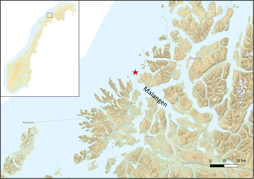
Figure 11. Map of Malangen fjord in Troms (northern Norway, 69°N), where the incubation experiment was performed in August 2017 (indicated by the red star). The incubation experiment was performed to measure the production of dissolved organic matter (DOC) in tangle kelp (Laminaria hyperborea). The incubation bags are shown in Figure 12.

Figure 12. The in-situ incubation of intact, young tangle kelp lamina (Laminaria hyperborea) with the purpose of measuring the export of dissolved organic carbon (DOC). The experiment took place in Malangen (Troms, northern Norway, 69°N) in August 2017. Photo: Karen Filbee-Dexter.
Results and discussion
Long-term storage (sequestration) of kelp POC in sediments
Station 38 had the highest sediment content of organic carbon, total carbon and chlorophyll a (Figure 13). This is the southernmost and shallowest station, and is located in a more sheltered area compared to the other stations. This station is located in an area of flat seabed and not in a depression where sediments are expected to accumulate at a higher rate. However, it is closer to the islands of Frøya and Hitra and may therefore receive higher input of kelp organic matter and terrestrial run-off. The higher content of fine-grained sediments (mud and clay) at stations 36 and 38 (Table 4), which are both located in the southern part of the sampling area, also indicates that this area is more sheltered and less affected by currents, resulting in higher settlement of both organic matter and inorganic particles.
The other three stations had a roughly similar content of organic carbon, total carbon and chlorophyll a (Figure 13). The core profiles suggest a relatively uniform distribution of organic carbon and total carbon from surface to 40 cm sediment depth, except for a strong increase in total carbon below 18 cm depth at station 36. These specific increase concentrations were discarded for further analyses, likely due to a method error or a body of organic matter buried in the sediments (like an animal carcass or massive deposition of macroalgae). The chlorophyll a content decreased rapidly from the surface sediments down to 5–10 cm depths. Below 10 cm depth, chlorophyll a concentrations were constant or decreased slowly, corresponding to the lower limit of the bioturbated zone (the zone in which seafloor fauna turn over the sediments on a regular basis in search for food and shelter).
Station 36 had the lowest mass sedimentation rates, followed by stations 34 and 38. Station 31 had a very high sedimentation rate in the surface sediment (0–1 cm), and then decreased rapidly for the lower sections of the core.


Figure 13. The concentration of a) total organic carbon, b) total carbon, c) chlorophyll a and derivatives (termed dev in the plot title, i.e. chlorophyll a break-down products), and d) mass sediment accumulation rates (lower right) in the sediment plotted against sediment depth in the cores from the four stations in Frohavet, Trøndelag (NW coast of Norway, 63–64°N). The stations are described in more detail in Figure 8 and Table 3. The extreme values for total carbon content (b) at station 36 (> 80 g C kg-1) was assumed to be an analytical error and discarded from further analysis.
| Sediment parameters | #31 | #34 | #36 | #38 |
| % < 0.063 mm | 49.3 | 50.5 | 71.7 | 65.2 |
| % > 0.063 mm | 7.4 | 6.3 | 10.4 | 17.5 |
| % > 0.125 mm | 13.2 | 13.5 | 13.0 | 14.9 |
| % > 0.25 mm | 10.9 | 11.9 | 3.8 | 2.2 |
| % > 0.5 mm | 7.5 | 8.9 | 0.5 | 0.2 |
| % > 1 mm | 6.0 | 4.0 | 0.5 | 0.1 |
| % > 2 mm | 5.7 | 4.8 | 0.0 | 0.0 |
| Mean particle size (φ) | 3.7 | 3.8 | 5.0 | 4.9 |
| Size class | Very fine sand | Very fine sand | Silt | Silt |
Table 4. Sediment characteristics including grain size distribution, mean particle size (φ; measure of particle diameter) and sediment size classification, analyzed in a bulk sample of the top 5 cm layer of sediment from grab samples collected at the four stations in Frohavet, Trøndelag (NW coast of Norway, 63–64°N). The stations are described in more detail in Figure 8 and Table 3.
Sediment chronology estimated from 210Pb-analysis for each core is shown in Figure 14a. Station 31 experienced the highest sedimentation rate, with sediments dated to only 11 years old at 4-5 cm core depth and reaching an age of about 120 years old at 25 cm core depth, which is a high sedimentation rate for this type of coastal system. In contrast, sediments from station 36 were dated to be nearly 60 years at 4–5 cm depth, as a result of the low sedimentation rate (Figure 13). The extrapolation of the sediment ages (Figure 14b) further emphasizes the difference in sediment age for the different stations, as a result of the different sedimentation rates, giving a range from ~180 years to > 500 years at 30 cm depth in the sediment. Sediment age and carbon accumulation are key numbers for estimating the sequestration of organic carbon from blue forests in the seafloor.
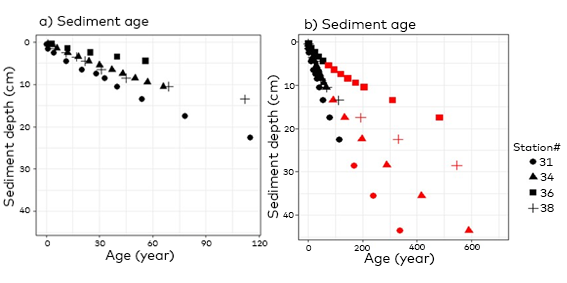
Figure 14. Age of sediment estimated from a) 210Pb-analysis of core sections and b) 210Pb-analysis of core sections (black data points) with sediment age extrapolated from 210Pb results assuming the same sedimentation rate as for the last 120 years (red data points). The data are retrieved from the four stations in Frohavet, Trøndelag (NW coast of Norway, 63–64°N), described in more detail in Figure 8 and Table 3.
The average mass sedimentation rate (MAR) for each core was calculated as an average of the sedimentation rates for sections below 2 cm core depth (Table 5). The upper 2 cm of the sediments was excluded to avoid the bioturbated zone, where sediments are physically mixed by living fauna. The linear sediment accumulation rate (SAR) was calculated by dividing the sediment depth of the deepest dated section by the age of the deepest dated section. Both mass and linear sediment accumulation rates were highest at station 31 and lowest at station 36.
| Station # | MAR (kg m-2 y-1) | LAR (cm y-1) | TOC < 2 cm (mg C/g) | C sequestration rate (g C m-2 y-1) |
| 31 | 1.03 | 0.19 | 29.3 | 31.1 |
| 34 | 0.82 | 0.16 | 29.3 | 26.8 |
| 36 | 0.53 | 0.08 | 34.3 | 14.9 |
| 38 | 0.98 | 0.12 | 49.6 | 49.5 |
Table 5. Average mass (MAR, kg m-2 y-1) and linear (LAR, cm y-1) sediment accumulation rates, total organic carbon (TOC) content in sediments and carbon sequestration rates (g C m-2 y-1) for the cores from the four stations in Frohavet, Trøndelag (NW coast of Norway, 63-64°N), described in more detail in Figure 8 and Table 3. MAR, LAR and TOC are the average of all sediment depths below 2 cm.
The organic carbon sequestration rate (g C m-2 y-1) was calculated for each section of the core as a product of the mass sediment accumulation rate (kg m-2 y-1) and organic carbon content in the sediments (g C kg-1):
Organic carbon sequestration rate (g C m-2 y-1) = sediment accumulation rate (kg m-2 y-1) x sediment TOC (g C kg-1)
Only organic carbon concentrations below 2 cm depth were included, in order to avoid the surface sediments which are most likely to be influenced by bioturbation and remineralization. The carbon accumulation rate was highest at station 38 and lowest at station 36 (Table 5), and station 31 and 34 had intermediate rates.
The amount of organic carbon sequestered is the product of sediment accumulation and organic carbon content. Other factors like bioturbation and oxygen content also affect the fraction of carbon being sequestered, but the most important factor is the delivery of inorganic particles that results in sediment accretion, as particulate organic carbon is mainly associated with mineral surfaces (Middelburg, 2019). This is evident in our results (Table 5): Station 38 (the shallowest station) had the highest carbon accumulation rate as a result of a high organic carbon content and relatively high sedimentation rates. Station 36 (354 m depth) on the other hand had a high organic carbon content in the sediments, but very low sedimentation rates, resulting in low carbon accumulation rates. Stations 31 and 34 (the deepest stations, depth > 500 m) had intermediate carbon accumulation rates as a result of high sedimentation rates but a lower organic carbon content.
Our results for organic carbon sequestration rates range from 14.9 to 49.5 g C m-2 y-1 (Table 5), and they are comparable to the results found for fjord environments in other studies. Smith et al. (2015) collated the results from a large number of globally distributed fjord samples and found mean organic carbon sequestration rates to range from 20–50 g C m-2 y-1 for all fjord regions except Alaska, which was more than 5 times higher. Other studies report similar numbers (Koziorowska et al., 2018; Winogradow & Pempkowiak, 2014). Organic carbon sequestration rates in fjords are reportedly higher than those of terrestrial forests, but lower than those of marine blue forests like salt marshes, mangroves and sea grasses (Mcleod et al., 2011). An overview of other studies reporting carbon sequestration in different areas and ecosystems is shown in Table 6.
| Area (marine sediments) | g C m-2 year-1 | References |
| Different fjord regions, globally | 20-50 | Smith et al. (2015) |
| Baltic Sea | 18-22 | Winogradow & Pempkowiak (2014) |
| Hornsund, Svalbard | 19.3.-30.3 | Koziorowska et al. (2018) |
| Kongsfjorden, Svalbard | 5.7-10 | Koziorowska et al. (2018) |
| UK (south) | 58.74 | Queirós et al. (2019) |
| Other ecosystems | ||
| Salt marshes | 218 ± 24 | Mcleod et al. (2011) |
| Mangroves | 226 ± 39 | Mcleod et al. (2011) |
| Seagrasses | 138 ± 38 | Mcleod et al. (2011) |
| Terrestrial forests | 4.0 ± 0.5 - 5.1 ± 1 | Mcleod et al. (2011) |
Table 6. Overview (with references) of reported carbon sequestration rates for different areas and ecosystems.
Genetic analysis (quantitative qPCR)
The purpose of the genetic analysis was to detect the presence of species-specific DNA from tangle kelp and sugar kelp in sediment cores in order to establish their presence and contribution to carbon sequestration. The aim was also to draft a preliminary, quantitative estimation. To this end, we developed and tested several specific qPCR assays for the two kelp species, shown in Figure 15, for asserting and tracking their presence in sediment cores and by doing so assess their contribution to carbon sequestration. Standard curves using calibrated reference material were used to roughly estimate kelp mass and hence carbon sequestration contribution in the sediments. To our knowledge, no species-specific qPCR assay has previously been developed for tangle kelp and sugar kelp.
The qPCR assay for tangle kelp showed excellent performance with an efficiency between 100.2% and 101.1%, and an R2 of 0.999. The sugar kelp assay was less performant with an efficiency around 77% and an R2 of 0.993 (data not shown). Overall results for both species’ detection and relative amount of kelp quantified in species-specific DNA ng/g wet sediment samples are shown in Figure 16, in all sampled cores as a function of age (year of sedimentation). Total unspecific DNA concentrations measured in the extracted core samples are shown in Figure 17. Results for each species individually as a function of a sample position in the core are shown in Figure 18 and Figure 19.
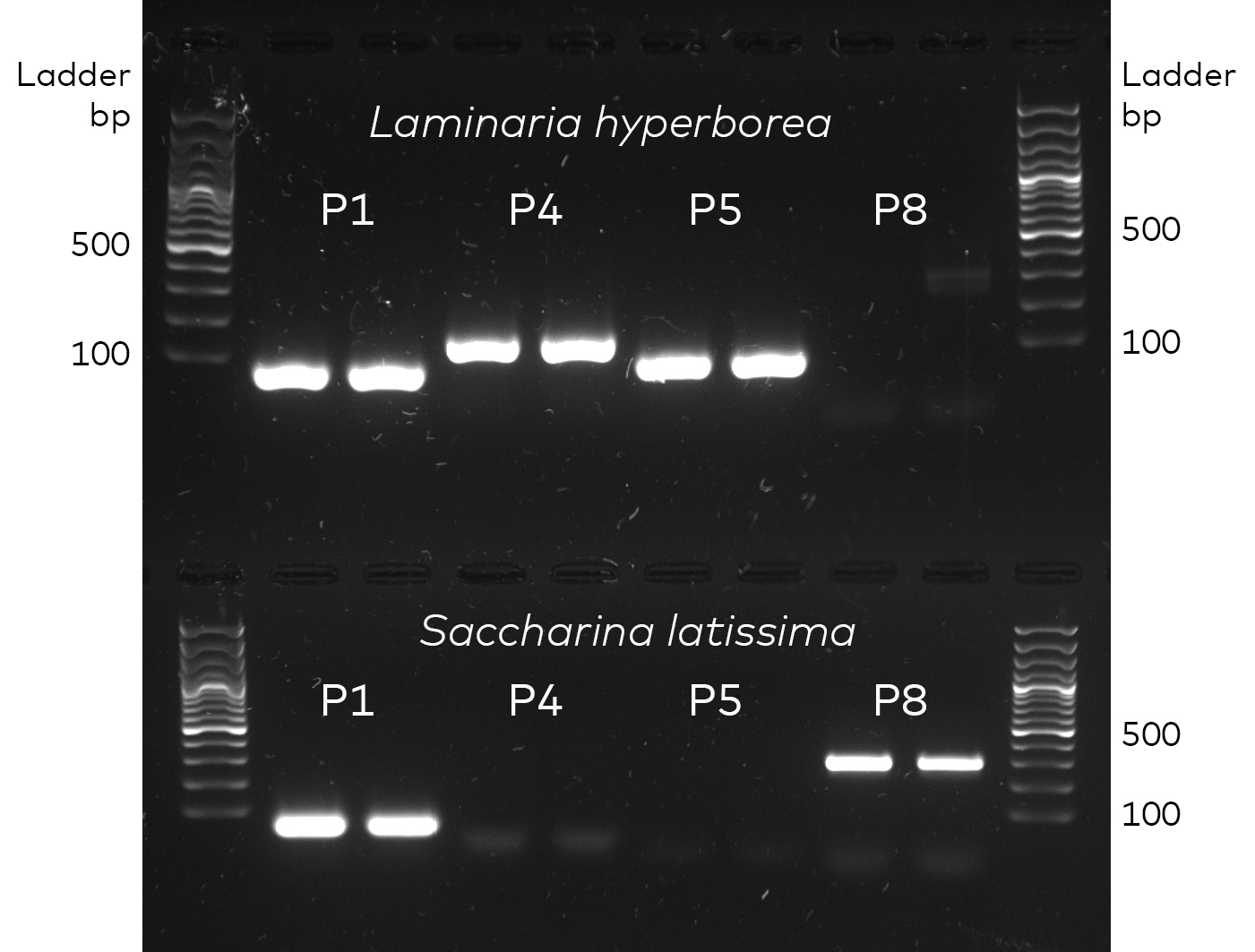
| Primer | Target | Amplicon size (bp) | Reference |
| P1 | Ectocarpales & Laminariales | 72 | Gachon et al., 2009 |
| P4 | Laminaria hyperborea | 144 | NIVA |
| P5 | Laminaria hyperborea | 88 | NIVA |
| P8 | Saccharina latissima | 312 | NIVA |
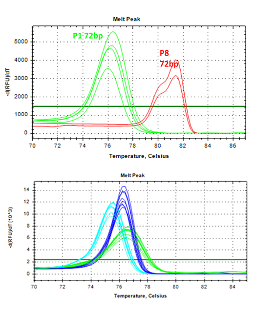
Figure 15. Test results for the species-specific qPCR (quantitative Polymerase Chain Reaction) assay for tangle kelp (Laminaria hyperborea) and sugar kelp (Saccharina latissima), showing strong and specific detection of the two kelp species. The P1 primers for Ectocarpales (a group of brown algae) were initially evaluated but not kept for analysis of the samples. Right side plots are melting point peaks characteristic for each assay. See text for more details.
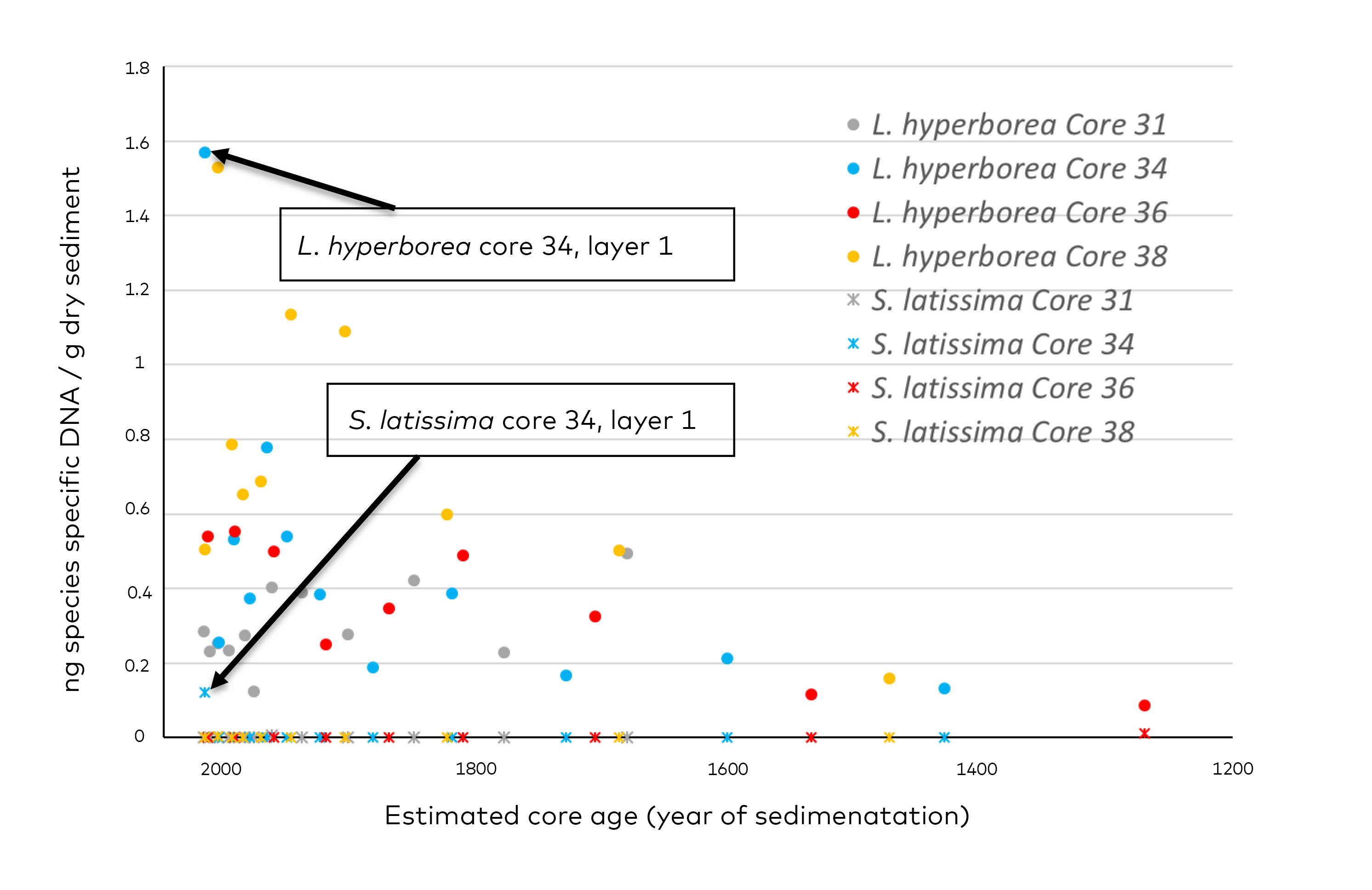
Figure 16. The DNA-specific detection, measured as the proportion of species-specific DNA (ng DNA per g dry sediment) for tangle kelp (Laminaria hyperborea) and sugar kelp (Saccharina latissima) against the estimated age of the sediments in the cores from the four stations in Frohavet, Trøndelag (NW coast of Norway, 63-64°N), described in more detail in Figure 8 and Table 3. Highest DNA concentration for both kelp species is found in the same sample (Core 34, layer 0–1 cm).
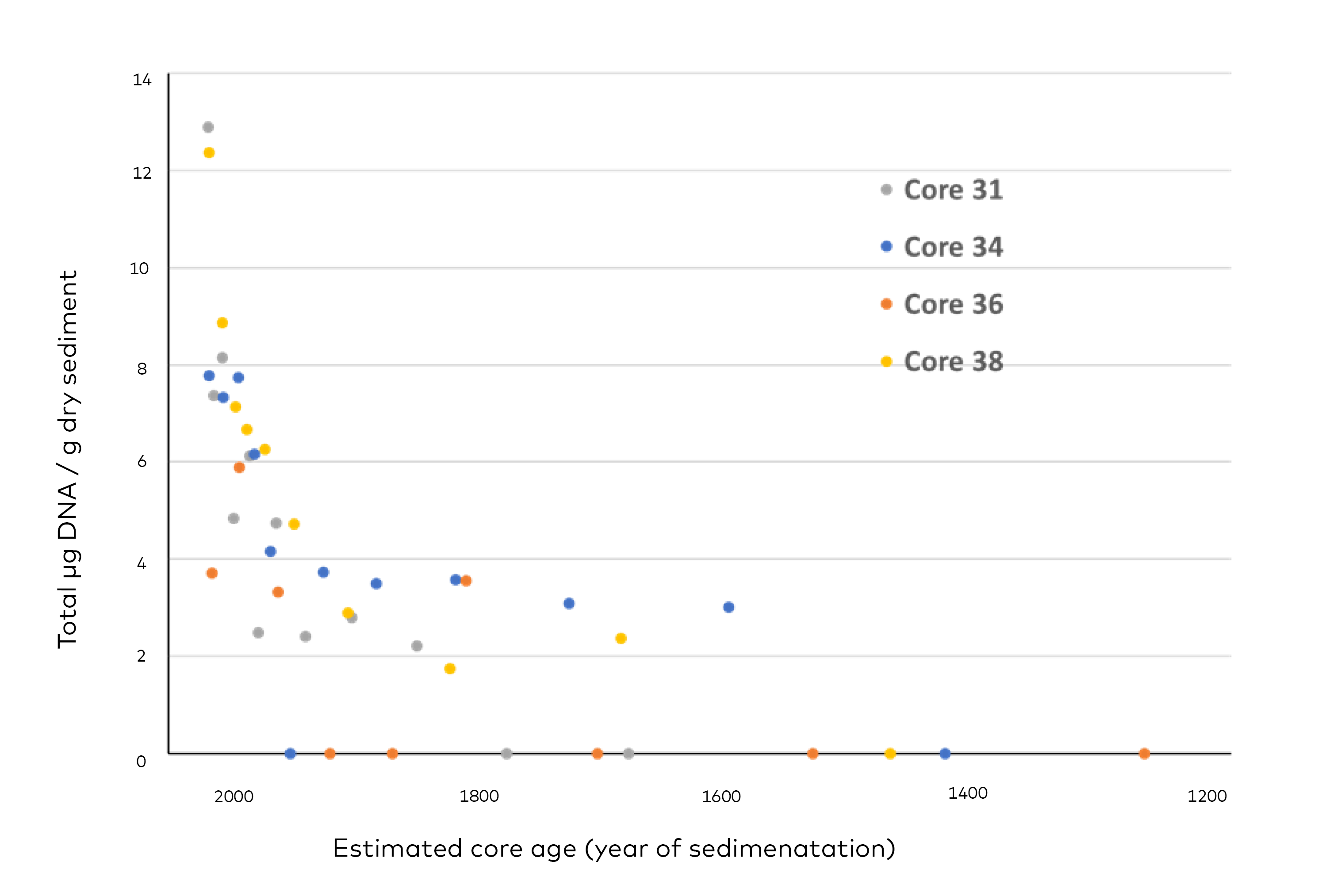
Figure 17. Total unspecific DNA concentration (µg DNA per g dry sediment) against the estimated age of the sediments in the cores from the four stations in Frohavet, Trøndelag (NW coast of Norway, 63–64°N), described in more detail in Figure 8 and Table 3. A cut-off value of 4 ng/µL was used for the measurements performed using NanoDrop™. Measurements under the cut-off (4 ng/µL) are considered unreliable and therefore plotted as "0".
The DNA analysis showed presence of tangle kelp in practically all collected cores. A general pattern was a decrease in the relative quantity with increasing depth in the core and thus with age of the sediment layer. In contrast to tangle kelp, sugar kelp was only detected in a few samples (Figure 18 and Figure 19). This could indicate a much lesser presence of sugar kelp in these coastal sediments, which possibly indicates that sugar kelp is consumed and degraded much more efficiently than tangle kelp, either prior to settling on the seafloor (less material settle) or in the sediments after deposition. However, the lower qPCR efficiency as well as amplification of a larger amplicon for the sugar kelp qPCR assay, 312 base pair (bp), compared to the tangle kelp assay (88 bp), may possibly have biased the results towards less signal from sugar kelp relative to tangle kelp. Indeed, it has also been previously reported that most DNA fragments found in marine ancient sediments are less than 100bp (Lejzerowicz et al., 2013).
Two stations, #34 and #38, showed higher relative quantities, and in particular the first core layer (0-1 cm) at station 34 showed high relative quantities for both targeted species (Figure 18 and Figure 19). These trends were also observed with relative quantities of unspecific total DNA, decreasing with age of the core, indicating a general breakdown of with sediment age (Figure 17). The highest total DNA quantities, from the upper sediment layers, are within previously reported measures ranging from 0.6 to 24 mg DNA per g dry sediment (Dell'Anno et al., 1999).
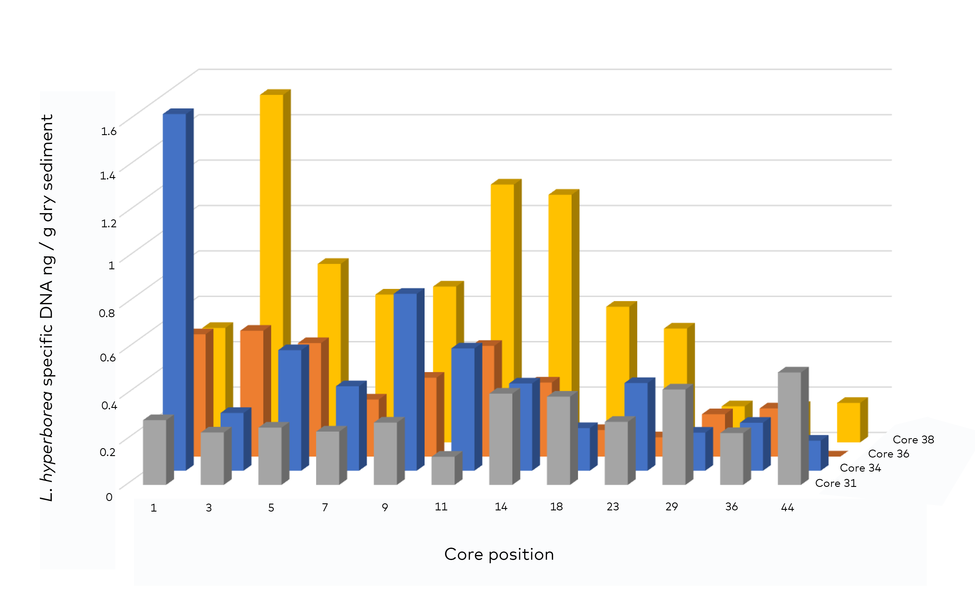
Figure 18. An estimate of the proportion of tangle kelp (Laminaria hyperborea) specific DNA (ng DNA per g dry sediment) for each core sample (i.e. the depth in the sediment core, in cm). The different colors represent the cores from the four stations in Frohavet, Trøndelag (NW coast of Norway, 63–64°N), described in more detail in Figure 8 and Table 3.
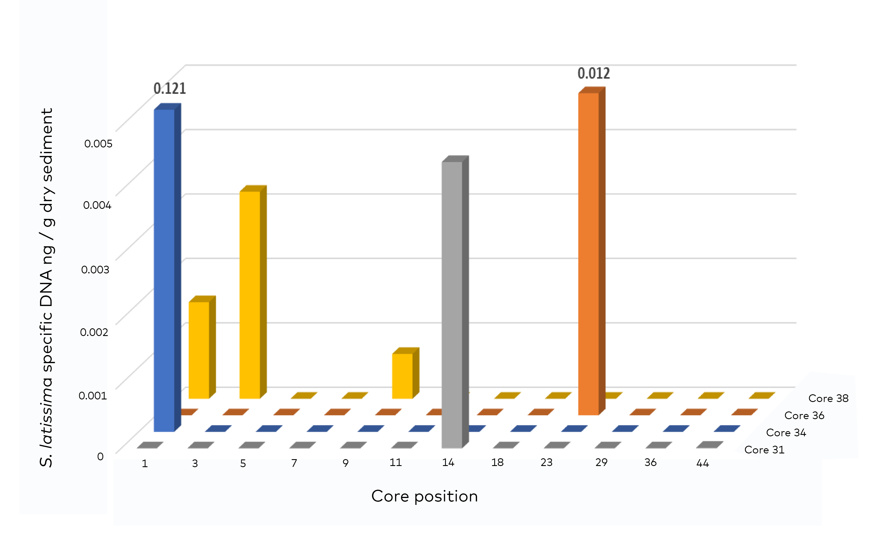
Figure 19. An estimate of the proportion of sugar kelp (Saccharina latissima) specific DNA (ng DNA per g dry sediment) for each core sample (i.e. the depth in the sediment core, in cm). The different colors represent the cores from the four stations in Frohavet, Trøndelag (NW coast of Norway, 63-64°N), described in more detail in Figure 8 and Table 3.
For kelp carbon quantification, the qPCR standard curves, built using serial dilution of standardized reference kelp DNA concentrations, are converted to mg organic carbon using the dry weight of DNA-extracted reference material. As extraction efficiency is likely to be higher for kelp material than for sediments, a correction factor of 10 was used. Another correction factor was added to take into account that DNA integrity, important for qPCR amplification, will degrade quicker than organic carbon. This point is exemplified in Figure 13, which shows relatively little variation between different core depths for TOC quantities, while total DNA consistently diminishes with increased core depths, as shown in Figure 17. By using a correction factor of 20 for this additional DNA degradation, the qPCR calculation for organic carbon quantities from tangle kelp varies from 10% to 32% of the measured TOC, as shown in Figure 20.
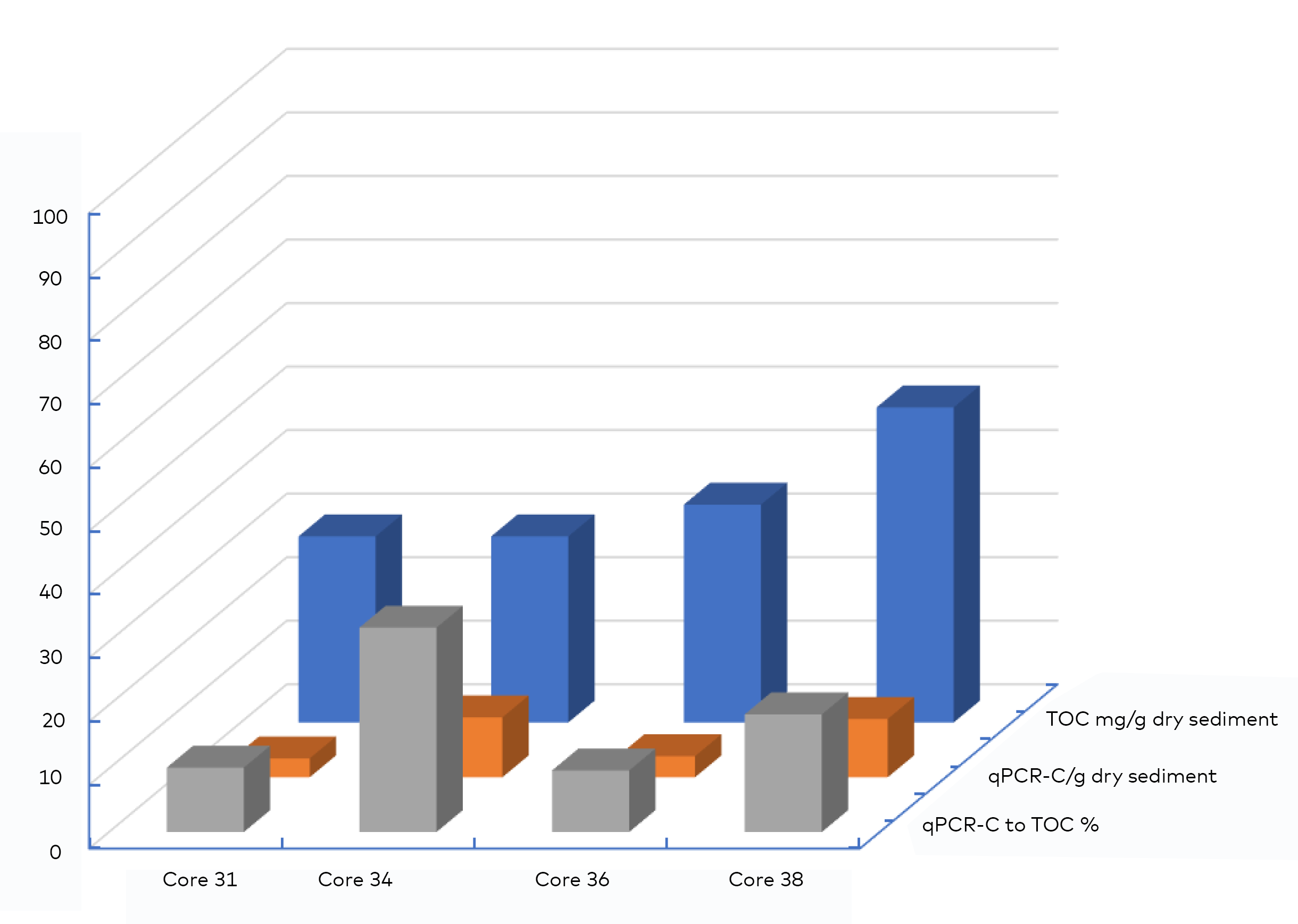
Figure 20. The blue bars show the total organic carbon (TOC) content (mg/g) measured in the sediment cores from the four stations in Frohavet, Trøndelag (NW coast of Norway, 63–64°N). The orange bars show an estimation of organic carbon from tangle kelp measured by species-specific qPCR. A correction factor was used for calculating this estimation (see text). The core position giving the highest qPCR measurement was used. Grey bars indicate the fraction (%) of the total organic carbon (TOC) that originates from tangle kelp.
The use of specific DNA to identify and quantify the contribution of macroalgae to carbon sequestration has recently been applied to seagrass (Reef et al., 2017; Hamaguchi et al., 2018). To our knowledge, the present study is the first to use species-specific qPCR assays to specifically evaluate the contribution of two kelp species to sediment carbon sequestration.
In recent years, the development of environmental DNA (eDNA) techniques has enabled new approaches to studying the origin and quantity of sequestered biological material in sediments (Lejzerowicz et al., 2013). For instance, eDNA has been used to distinguish autochthonous from allochthonous plant contribution in Australian marine sediments using Next Generation Sequencing (NGS) for metabarcoding. Here they concluded that seagrass represented 88% of the extracted eDNA, indicating a high fraction of seagrass organic carbon in the investigated sediments (Reef et al., 2017). Another eDNA metabarcoding study was able to identify the macrophyte contribution to blue carbon in the first centimeter of the upper layer of the sediments (Ortega et al., 2020a; Ortega et al., 2020b). Another study in Japan uses seagrass-specific probe qPCR and ddPCR assays for species identification and quantitative estimation of carbon sequestration in marine sediments (Hamaguchi et al., 2018). The present work is taking these studies further and applying it to two kelp species. Here we suggest a new method, and envision that this will improve the identification of organic carbon sequestration source and quantify the role of these macroalgae in marine organic carbon sequestration. The primers developed in this project will enable studies of specific ecosystem components and their importance to carbon sequestration, and pave the way for better marine carbon budgets.
Stable isotopes
Stable isotopes of carbon and nitrogen may be useful indicators of food origin and trophic levels. δ13C gives an indication of carbon source in an ecosystem, a food web, or a diet. For instance, it is possible in principle to detect differences in the importance of autochthonous (native marine) and allochthonous (watershed/origin on land) carbon sources in the food web, since the δ13C signature of the land-based energy sources is lower (greater negative number) than the autochthonous. Also, δ15N (although to a lesser extent than δ13C) may be lower in allochthonous organic matter than in autochthonous organic matter (Helland et al., 2002), but more importantly, it increases in organisms with a higher trophic level due to greater retention of the heavier isotope (15N). In the current context, it is of interest that kelp carbon has a higher δ13C signature than phytoplankton carbon (Dunton & Schell, 1987).
Isotopic ratios of carbon (δ13C; Figure 21) and nitrogen (δ15N; Figure 22) differed between stations, but also somewhat in sediment depth/age within stations. Generally, however, across the sediment ages, δ13C was highest at stations 31 and 34 (Figure 21), while δ15N was lowest at stations 31 and 34 (Figure 22). Note that sedimentation rates differed between stations (Figure 13), and similar sediment core depths between stations therefore had different ages.
The differences in sediment isotopic ratios between stations can also be seen from Figure 23, where δ15N is plotted against δ13C. Sediment sections from stations 31 and 34 are located at the lower right (higher δ13C and lower δ15N), while sediment sections from station 36 are located at the higher left (lower δ13C and higher δ15N). Apparently, the largest variation between sediment sections from the same core was at Station 38.
Compared with isotopic ratios in the kelp samples, the signatures in sediment sections from stations 31 and 34 showed the closest resemblance (higher δ13C and lower δ15N; Figure 24), suggesting that these stations are more influenced by organic matter originating from kelp than stations 36 and 38 with a higher content of phytoplankton-derived organic matter. This is based on kelp carbon having a higher δ13C signature than phytoplankton carbon (Dunton & Schell, 1987). These results partly support the conclusions from the DNA analysis, which showed the highest contributions of kelp at stations 34 and 38 (Figure 18). The combined result from the stable isotope and DNA analyses suggests that station 34 contained the highest content of kelp carbon, which supports the hypothesis that deep basins in coastal regions may work as accumulation hotspots for kelp organic matter.
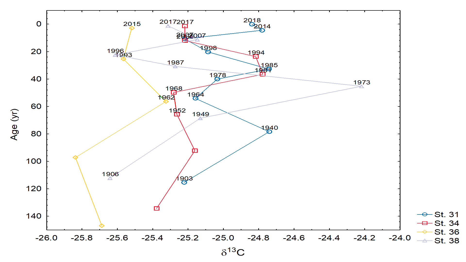
Figure 21. d13C in sediment core sections from four stations in Frohavet, Trøndelag (NW coast of Norway, 63-64°N), with increasing sediment age (top to bottom on the vertical axis; increasing with sediment depth). Sections were dated using 210Pb, and the results (year AD) from this dating are superimposed. For the data points not dated, the age is estimated from extrapolation. Available data from the last 150 years are included.
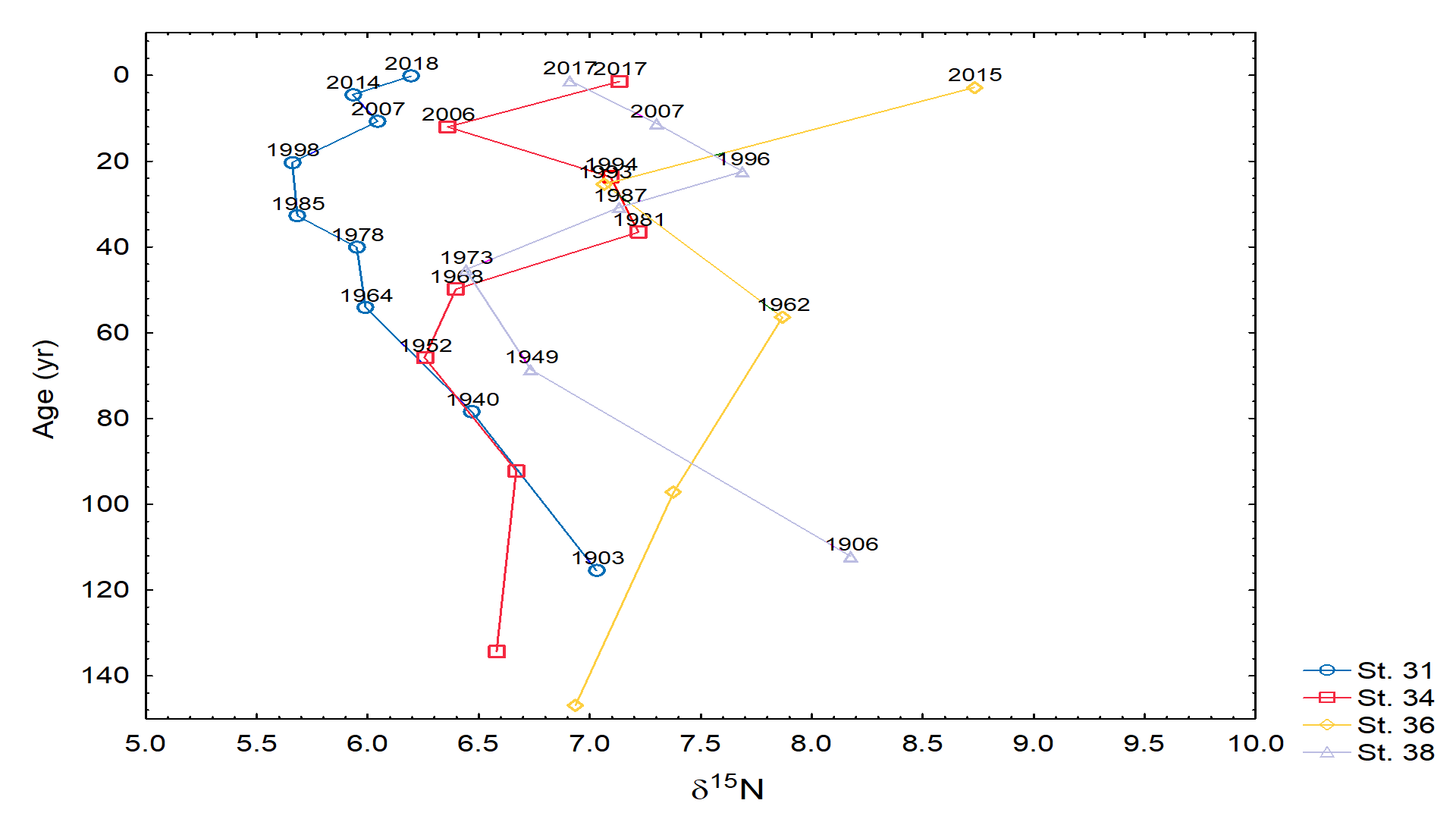
Figure 22. d15N in sediment core sections from the four stations in Frohavet, Trøndelag (NW coast of Norway, 63–64°N), with increasing sediment age (top to bottom on the vertical axis; increasing with sediment depth). Sections were dated using 210Pb, and the results (year AD) from this dating are superimposed. For the data points not dated, the age is estimated from extrapolation. Available data from the last 150 years are included.
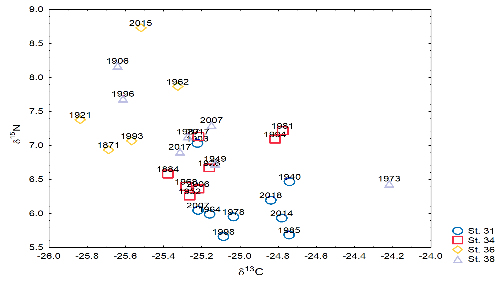
Figure 23. δ15N vs. δ13C in sediment core sections from the four stations in Frohavet, Trøndelag (NW coast of Norway, 63–64°N). Sections were aged (superimposed). Available data from the last 150 years are included.
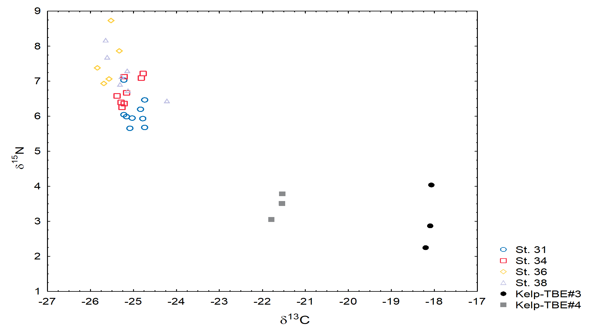
Figure 24. d15N vs. d13C in sediment core sections from the four stations in Frohavet, Trøndelag (NW coast of Norway, 63–64°N), and in samples of tangle kelp (Kelp-TBE#3, black points) and sugar kelp (Kelp-TBE#4, grey points) collected in 2018. Sediment sections aged < 150 years are included.
Export of dissolved organic carbon (DOC) from kelp
DOC export rates ranged from 10.1–13.2 µg g-1 blade fresh weight (FW) h-1, with a corresponding O2 production from 0.17–0.49 µmol g-1 blade FW h-1 (Figure 25). The kelp incubated in the dark had a minor DOC production (< 0.2 µg g-1 blade FW h-1) and a negative O2 production, representing the respiration and kelp metabolic activity during night hours. The kelp DOC production rate was highest at 5 m depth, but there seemed to be little difference in the DOC production at the different depths (1, 5 and 10 m).
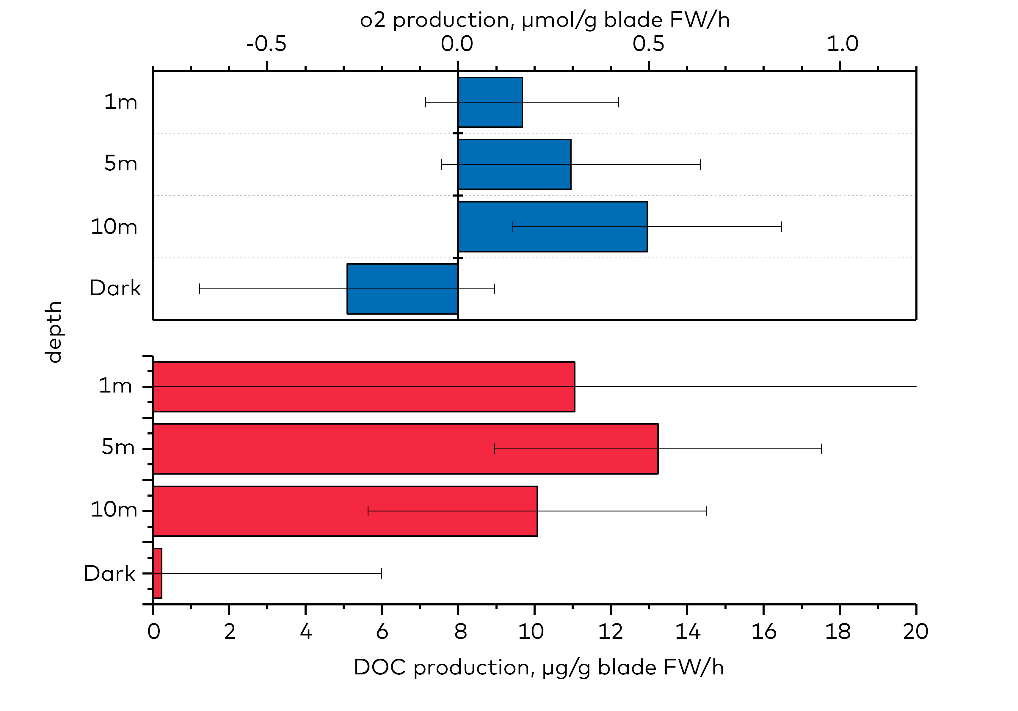
Figure 25. Production of oxygen (O2) in the upper graph (blue) and dissolved organic carbon (DOC) in the lower graph (red) estimated from in situ incubations of tangle kelp (Laminaria hyperborea) in transparent and gas-tight plastic bags at different water depths.
DOC production per fresh weight (FW) tangle kelp per hour was converted to gram carbon per square meter per year by correcting for the C:FW ratio (0.163 x 0.33, Pedersen et al., 2019), the kelp biomass per square meter, and assuming 16 hours of daylight per day, and an annual productive period of 210 days (March-September). Tangle kelp DOC production was estimated at 480–630 g C m-2 year-1 (Figure 26). This corresponded to a DOC production of 96–126% of the net primary production (NPP) of particular matter (biomass increase) at the study site on an annual basis (Annual DOC production m-2 h-1 = (µg C g-1 blade FW h-1) * 14 314 g FW kelp m-2 * 16 h * 210 d). This implies that when net primary production is measured from an increase in POC or from growth rates, it underestimates the “true” primary production by up to 100% if the DOC production is excluded.
A similar study that was conducted in May indicated a DOC production that was 83% larger than in August (Table 7). For further calculations, we take a conservative approach here and assume the DOC production to be 50% of the NPP. As clearly shown in Table 7, the DOC production is nevertheless uncertain and may represent one of the major uncertainties in the carbon budget for blue forests. Thus, we suggest further studies of macroalgae DOC production in order to improve future blue carbon budget assessments.
Figure 26. Annual tangle kelp (Laminaria hyperborea) DOC export rate estimated from DOC export measured 24 h in August 2017 in Malangen (Troms, northern Norway, 69°N).
An overview of other studies reporting DOC production from tangle kelp is given in Table 7. Seasonal differences in DOC production probably explain some of the differences in results across the studies. As shown in Abdullah & Fredriksen (2004), the DOC production is highest in spring (March–June) and lowest in autumn (August–October). Abdullah & Fredriksen (2004) reported a monthly mean of 1 029 g C m-2 year-1, whereas measurements taken in August (present study) and September (Barrón et al., 2014) are considerably lower, ranging from 134 to 480–630 g C m-2 year-1.
| Locality | Source data | DOC prodoction g C m-2 y-1 | DOC prodoction (in % NPP) | Comment |
| Malangen, Norway1 | 480–630 | 96–126 | August | |
| Malangen, Norway1 | 860–1 120 | 86–112 | May | |
| Møre og Romsdal, Norway2 | 1.29 kg C m-2 year-1 | 1 029 | 26 | Monthly mean |
| Trondheim, Norway3 | 30.6 mmol C m-2 d-1 | 134 | 30–45 | September |
| Scotland4 | 16.5 tonne hectare-1 year-1 | 800–1 650 | 3 and 9 m depth, sampled over 15 months | |
| Global mean5 | 101 (sd. 55) | 11–37 | ||
| Estimated average | 550–790 | 50–69 | ||
| 1 Present study; 2 Abdullah & Fredriksen, 2004; 3 Barrón et al., 2014; 4 Jupp & Drew, 1974; 5 Krause-Jensen & Duarte, 2016 | ||||
Table 7. Relevant studies with measures of tangle kelp (Laminaria hyperborea) DOC production and the DOC production as a percentage of the NPP. In this study we take a conservative approach and assume the DOC production to be 50% of the NPP for “average kelp forests”.
Conclusions
In this chapter we presented new data for long-term storage (sequestration) of kelp carbon from sedimentation in shelf sediments and through DOC production. The numbers were entered in the Nordic blue carbon budget (Chapter 3) and used to update estimates of the long-term storage of kelp carbon in marine sediments and in the deep sea.
Organic carbon sequestration and the fraction originating specifically from kelp was derived from sediment cores collected across a depth gradient in Frohavet in Mid Norway (242 to 531 m depth). The total organic carbon sequestration ranged from 15 to 50 g of carbon per square meter per year. Developing a species-specific DNA-based diagnostic assay enabled us to trace kelp-specific DNA and quantify the fraction of kelp as a percentage of the total organic carbon in the sediments. This fraction was 10–32%, which supported a kelp carbon sequestration rate of 13 g of carbon per square meter per year in shelf sediments.
The method documented the presence of tangle kelp and sugar kelp in seafloor sediment and showed that kelp was present in practically all layers of the collected sediment cores (down to 23 cm/120 years old). This is one of the first attempts to develop and apply species-specific qPCR assays to trace kelp DNA in marine sediments, and the first time this has been achieved in Norway. We anticipate that this method will enable the tracing of organic carbon from kelp and other macroalgae in seafloor sediments, and thereby improve our understanding of the role of kelp and blue forests in the marine carbon cycle and their potential for long-term carbon storage.
The production of dissolved organic carbon (DOC) from tangle kelp was measured during a field (in situ) incubation experiment in Malangen in northern Norway. The annual DOC production from kelp was estimated at 860–1 120 g and 480–630 g of carbon per square meter per year in May and August, respectively. This corresponded to a DOC production similar to the net primary production (NPP) of particulate matter, i.e. equivalent to the growth rate of kelp biomass annually. As a percentage of NPP, the DOC production was 86–112% in May and 96–126% in August, respectively. The results demonstrate that kelp forests produce large quantities of DOC in addition to the biomass production, as also shown in previous studies. The DOC production is excluded from most production measures and largely ignored in estimates of blue forest net primary production measures. The “true” net primary production is therefore underestimated.
Despite the efforts of this project, the rates of both seafloor carbon sequestration and DOC production are major uncertainties in Norwegian, Nordic and global carbon budgets. This is because there is a large variation between species and ecosystems, and across seasons, water depth and latitude (water temperature). However, in this work we report on the first kelp-specific carbon sequestration rates carried out in Norway and have added to existing Nordic literature on DOC production from kelp, which is a step in the right direction. To further improve the estimates of carbon sequestration from Nordic blue forests, further efforts and resources are needed to improve data availability and assess uncertainties across the Nordic habitats. This should include the determination of carbon sequestration in seafloor sediments along the Nordic coasts and offshore, DOC production in kelp, rockweed and seagrass and its export and long-term fate (break down or sequestration), and the export and fate of POC from coastal habitats to deep sea regions.
The rates derived during fieldwork in this project were collected across different seasons and locations, restricted by the budget and logistics available. In order to complete the Norwegian and Nordic blue carbon budgets (Chapter 3), we have extrapolated these (often local) data, to our best knowledge, to be representative across regions and seasons through analysis and comparison with existing literature.
Chapter 3 – Nordic blue carbon budget
Vegetated coastal habitats have been recognized as important for various ecosystem services, including removal of carbon from the biosphere, i.e. carbon sequestration or so-called natural carbon sinks (Duarte et al., 2005; Nellemann et al., 2009; Mcleod et al., 2011). Historically, kelp and macroalgae were not considered to contribute to blue carbon sequestration because they live on hard-bottom substrates (Nellemann et al., 2009), however there is increasing evidence that significant amounts of carbon from these habitats are transported, buried and potentially sequestered in coastal and deep-sea sediments (Krause-Jensen & Duarte, 2016; Pessarrodona et al., 2018; Fillbee-Dexter et al., 2019; Pedersen et al., 2019). Nevertheless, there is still considerable uncertainty about the overall carbon budget of blue forests (kelp, seagrass and rockweed), and the magnitude and significance of the standing stock (in living biomass) and sequestration of carbon, both on a global and regional scale.
The aim of this chapter is to provide an update on the marine blue carbon budget with respect to contributions of kelp, rockweed and seagrass in order to estimate the potential for blue forest carbon sequestration in the Nordic region. Here we present quantitative estimates for each of the blue forest habitats, with rates for net primary production (NPP), transport and export of carbon, and the carbon sequestration in shelf sediment, seagrass meadows and to the deep sea (below 1 000 m water depth). The outcome of this chapter is the first comprehensive carbon budget for Nordic blue forests and their joint contribution to the sequestration of carbon, and thus the ability of these systems to act as natural sinks of carbon.
Methods
The carbon budget for Norwegian kelp forests is based on the modelling efforts in Chapter 1, empirical findings in Chapter 2, and values from the scientific literature. Where possible, rates were derived from studies from the Norwegian and/or Nordic region. The carbon budget model was largely adopted from Krause-Jensen & Duarte (2016) and modified to Norwegian and Nordic conditions and regions where needed, depending on data availability. The two species of kelp included in the study; tangle kelp (Laminaria hyperborea) and sugar kelp (Saccharina latissima), were assumed to have identical rates of NPP, production of particulate organic carbon (POC) and dissolved organic carbon (DOC), carbon export from habitats, and sequestration potential per unit area. The carbon budget for rockweed was synthesized using the same calculation model as for kelp but with specific rates for rockweed NPP, POC and DOC production. Export and sequestration, burial rates in shelf sediments and rates of export to deep sea systems were assumed to be similar to the pathways for kelp, assuming similar physical properties and biochemical composition of the biomass. The carbon budget for seagrass was based on a model by Duarte & Krause-Jensen (2017), with rates of NPP and carbon sequestration from Danish and Nordic studies. See the individual sections below for details on each of the processes in the carbon budget. Because of the huge uncertainty in the areal estimates for the blue forest’s habitats in Greenland, Greenland was excluded from the Nordic carbon budget. Proximate numbers for Greenland are given separately.
Results and discussion
The following sub-chapters will revise the major processes and pathways involved in establishing an overall carbon budget for the Nordic region, i.e. the net primary production, transport and export of carbon from the habitats, and the sequestration of carbon in shelf and deep sea water and sediments (see schematic overview in Figure 27). Finally, an updated carbon budget for Nordic blue forests is presented (Figure 29, Figure 30).
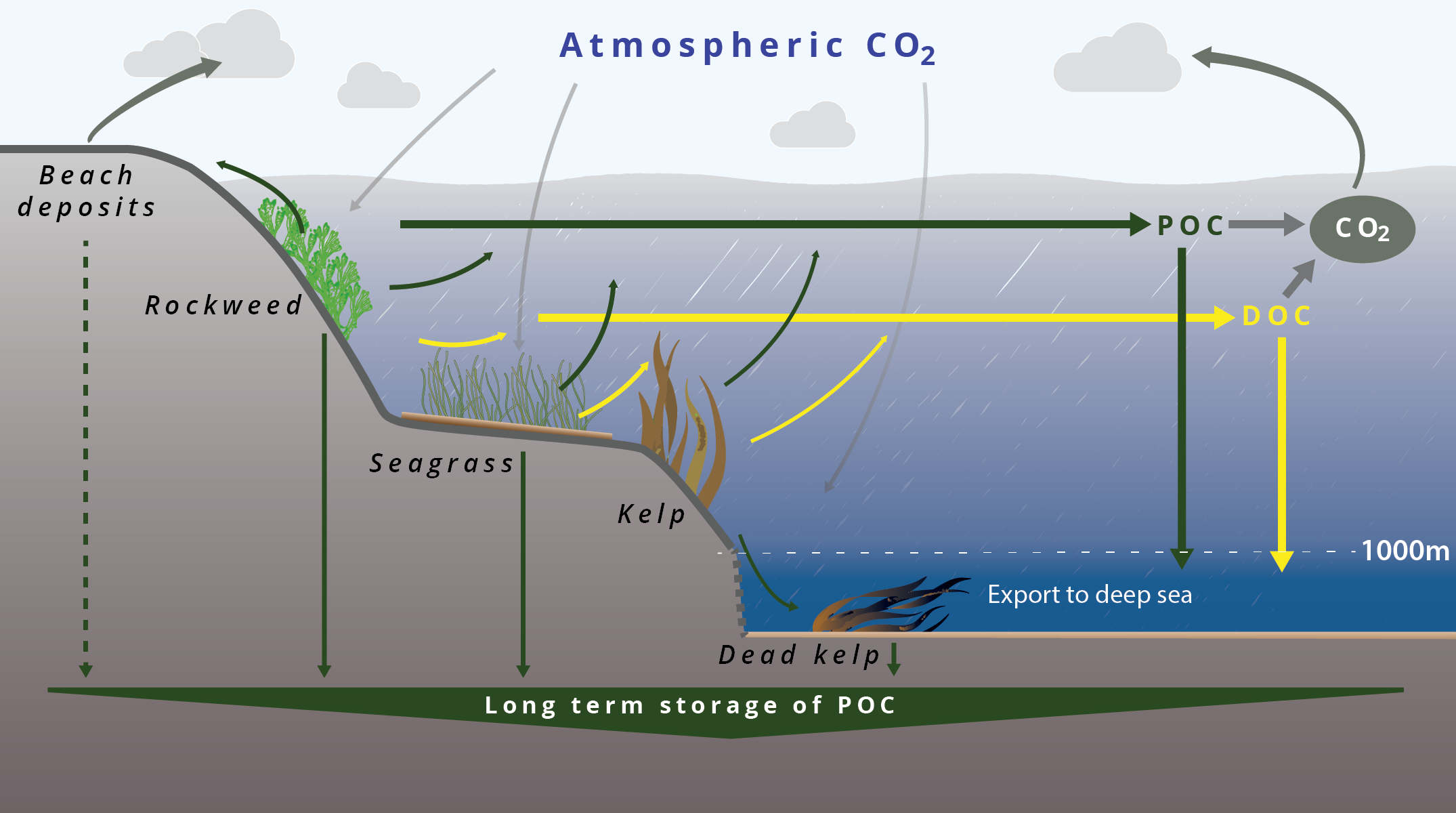
Figure 27. Schematic overview of key carbon pools and fluxes in the Nordic blue carbon budget, including kelp forests, rockweed beds, and seagrass meadows. The particulate organic carbon (POC) and dissolved organic carbon (DOC) production and export from each habitat to the shelf and deep sea (below 1 000 m water depth) is indicated.
Net primary production in the blue forest habitats
We compiled areal rates of net primary production (NPP) for kelp forests, rockweed beds and seagrass meadows from across the Nordic region as input to the carbon budget. Rates are given per square meter and compiled for Norway and the Nordic region (Table 8), and Greenland separately due to the large uncertainty in the numbers (Table 9). NPP rates per unit square meter or equivalent areal units have frequently been measured under various conditions and regions. Thus, NPP data are relatively abundant and consistent relative to other figures in the carbon budget, both regarding the Nordic region and globally.
The annual NPP for kelp forests in Norway was estimated at 309 (147–581) g C m-2 y-1. The estimate is based on average production measures for individual plants of tangle kelp in Northern and Western Norway (Abdullah & Fredriksen, 2004; Pedersen et al., 2012; Pedersen et al., 2019; Sjøtun et al., 1995), and corrected according to the total modelled Norwegian NPP divided by the predicted area (Chapter 1). Total NPP for the Norwegian kelp forest was estimated at 2.3 million tonne C y-1 (2 292 Gg C y-1), while the sum for Nordic kelp was 3.4 million tonne C y-1 (3 396 Gg C y-1, Table 8). NPP per unit area was assumed to be the same for the two kelp species (tangle kelp and sugar kelp).
The annual NPP for rockweeds was estimated at 292 ±- 279 g C m-2 y-1 representing averaged reported rates from Denmark and Finland (Attard et al., 2018; Attard et al., 2019; Krause-Jensen et al., 2012; Pedersen et al., 2005), corresponding to a total Nordic rockweed NPP of 1.6 million tonne C y-1 (1624 Gg C y-1, Table 8).
The annual NPP for seagrass was estimated at 326 ±- 115 g C m-2 y-1 representing averaged rates from Denmark and Finland (Krause-Jensen et al., 2012; Röhr et al., 2016 and references herein), corresponding to a total Nordic seagrass NPP of 0.85 million tonne C y-1 (850 Gg C y-1, Table 8). To summarize, the Nordic blue forests represent an NPP in the order of 5.9 million tonne C y-1 (5 870 Gg C y-1, Table 8). This is equivalent to approximately 1% of the global blue forest NPP (0.68 Pg y-1, Duarte & Krause-Jensen, 2017) and about 0.1 ‰ of the entire global marine primary productivity (i.e. 50 Pg C y−1 (1 Pg or 1 Gt is 1015 g).
To convert rates of production and export between fresh weight (FW), dry weight (DW) and carbon content (C), we applied average values from the literature, i.e. for kelp and seaweeds ratios for DW:FW of 0.15 and C:DW of 0.31 (Norwegian data from the KELPEX project) (Pedersen et al., 2019), and for seagrass, a ratio of 0.38 was applied for C:DW (Atkinson & Smith, 1983; Krause-Jensen et al., 2012).
Table 8. Compiled estimates of area, biomass, net primary production (NPP), and carbon sequestration rates (carbon sequestration) for both particulate organic matter (POC) and dissolved organic matter (DOC) per square meter, for Norway, and for the Nordic region (excluding Greenland). Carbon sequestration rates are given in units of giga gram C and CO2 equivalents. Estimates are predicted or are the weighted average of available data. The brackets indicate range (min-max) or standard deviation (SD). Details in appendix B.
| Areal units | Habitat | Area predicted | Carbon stocks | NPP | Carbon sequestration rate (POC, DOC) | ||
km2 | Living biomass g C m-2 | Sediment stocks g C m-2 | g C m-2 y-1 | g C m-2 y-1 | - | ||
| m2 | Kelp forests a | 1 | 670 | 0 | 309 (147–581) | 67.8 (19–81) | - |
| Rockweed b | 1 | 300 (150–500) | 0 | 292 (279) | 37.8 (11–45) | - | |
| Seagrass c | 1 | 79 (71–87) | 2 600 (700–4 500) | 326 (115) | 51 (14) | - | |
| km2 d | Gg C | Gg C | Gg C y-1 | Gg C y-1 | Million tonne CO2 equiv. y-1 | ||
| NORWAY | Kelp forests | 7 417 (5 933–9 317) | 4 969 | - | 2 291 (1 090–4 309) | 503 (141–601) | 1.8 |
| Rockweed | 3 090 | 927 | - | 903 (862) | 117 (33–139) | 0.4 | |
| Seagrass | 90 | 7 | 245 | 29 (10) | 4.6 (1.3) | 0.02 | |
| Total | 10 597 | 5 904 | 245 | 3 223 | 625 | 2.3 | |
| NORDIC | Kelp forests | 10 990 (9 252–15 908) | 7 363 | - | 3 396 (1 665–6 385) | 746 (209–891) | 2.7 |
| Rockweed | 5 556 | 1 667 | - | 1622 (1550) | 209 (58–249) | 0.8 | |
| Seagrass | 2 611 | 206 | 6 789 | 850 (300) | 133 (37) | 0.5 | |
| Total | 19 157 | 9 236 | 6 789 | 5 868 | 1 088 | 3.9 | |
| a Biomass from Gundersen et al. (submitted), NPP predicted in WP1 (based on Abdullah & Fredriksen., 2004; Pedersen et al., 2012; Pedersen et al., 2019; Sjøtun et al., 1995), C sequestration calculated from model by Krause-Jensen & Duarte (2016), see details in text and Appendix B b Biomass from Attard et al. (2018), NPP (Pedersen et al., 2005; Attard et al., 2019; Attard et al., 2018; Krause-Jensen et al., 2012), C sequestration calculated from model by Krause-Jensen & Duarte (2016), see details in text and Appendix B c Biomass (Röhr et al., 2018), NPP (Krause-Jensen et al., 2012; Röhr et al., 2016), and sequestration from Röhr et al. (2016) (average Denmark) d Area from WP1 | |||||||
Table 9. Compiled estimates of area, biomass, net primary production (NPP), and carbon sequestration rates (C seq.) for both particulate organic matter (POC) and dissolved organic matter (DOC) for Greenland. Carbon sequestration rates are also given in units of CO2 equivalents. Estimates are based on averaged rates per meter from Table 8. These numbers include huge uncertainty both regarding the areal coverage and the estimated rates due to very limited data availability, and are therefore excluded in the carbon budget for the Nordic region. Estimates are predicted or are the weighted average of available data. The range (min-max) is shown in brackets. See details in Appendix B.
| Areal units | Habitat | Area predicted | Carbon stocks | NPP | Carbon sequestration rate (POC, DOC) | ||
km2 | Living biomass Gg C | Sediment stocks Gg C | Gg C y-1 | Gg C y-1 | Million tonne CO2 equiv. y-1 | ||
| Greenland | Kelp forests | 2 6704 (24 493–31 700) | 17 892 | - | 8 252 (3 925–15 515) | 1 812 (508–2 164) | 6.5 (1.8–7.8) |
| Rockweed | - | ||||||
| Seagrass | - | ||||||
| Total | 2 6704 | 17 892 | - | 8 252 | 1 812 | 6.5 | |
Detritus formation and carbon export
In this study we define the export production as the dissolved and particulate carbon (DOC + POC) that is transported and removed out of the blue forest habitat. The fate of this exported carbon can be POC sequestration in the form of long-term carbon stored in the sediments, DOC sequestration through export below the ocean mixed zone to deep water masses (> 1 000 m depth), or emission to the atmosphere as CO2.
In kelp forests, large amounts of kelp particulate matter are produced and eventually detached from living biomass and exported as detrital matter, where the carbon fraction is termed particulate organic carbon (POC). The major processes are through detachment of entire plants or blades after storm events or at the end of the life cycle or as blade erosion, which is a running process. The formed detritus is then exported out of the forest, where it supports secondary production (grazing and remineralization) or contributes to long-term storage of blue carbon through permanent burial in the seafloor (Figure 29).
In a study of kelp forests of northern Norway, the authors found that >50% of the total detrital production was due to the detachment of old blades. In addition, dislodgement of whole plants and/or blades corresponded to 24% of the detritus production, while distal blade erosion accounted for 23%. In total, the formation and export of kelp detritus came to 478 ± 41 g C m−2 year−1 (96% of the NPP) (Pedersen et al., 2019). These rates are comparable to data on detritus production measured in the north of Scotland (Pessarrodona et al., 2018), but lower than most other places. Here we adopted the rates from Pedersen et al. (2019) and normalized them to NPP, representing the only direct quantification of detritus formation in Norwegian kelp forests. Upscaled for this study, this corresponds to a Norwegian kelp forest detritus formation of ~1.1 million tonne C per year, for tangle kelp alone (and approximately the same for sugar kelp). For simplicity, we adopted the same parameters for sugar kelp and rockweed in further calculations of detritus formation and carbon export.
Seagrass meadows have been shown to export a substantial portion of their production, however most studies have focused on burial of organic matter inside the meadows, leaving the export production of POC out of the meadows largely unaccounted for in terms of carbon budgets and estimates of long-term storage. Recently, Duarte & Krause-Jensen (2017) showed that the export production accounts for a significant part of the NPP (24%) and that the POC export alone accounts for ~18% of the total long-term storage of carbon for seagrass, based on a global data assessment. Here we applied these figures to the Nordic carbon budget, assuming that the numbers for export and transfer into other habitats comply with the global scheme. Figure 28 provides examples of particulate matter export from various habitats to illustrate the range of detritus production in blue forests and related habitats (adopted from Pedersen et al., 2019)
Figure 28. The amount of carbon (measured as production per m2 per year) originating from different habitats, illustrating the relatively large amount of detritus exported from rockweeds (here termed Non-kelp seaweeds), seagrasses and kelps relative to phytoplankton and terrestrial habitats. Asterisks indicate significant differences compared to kelp. Figure redrawn from Pedersen et al. (2019).
A fraction of the inorganic carbon fixed during photosynthesis in kelp, seaweeds and seagrass is released during growth as dissolved organic carbon (DOC). A part of the released DOC (emitted from the organisms) supports the microbial loop and is consumed by microorganisms (mainly bacteria). The remainder contributes to long-term storage of carbon if refractive (not available to the food web), and/or if transported below the mixed zone of the large oceans below 1 000 m water depth, as suggested by Krause-Jensen & Duarte (2016).
Since there are still large uncertainties regarding estimates of the production and fate of DOC from kelp and seaweeds, we included a field study to provide Norwegian kelp-specific rates of DOC production to support the limited literature available, see Chapter 2. In this study, we found a DOC production from kelp of 480–1 120 g C m-2 y-1 (Table 7). These values support previous estimates and fall within the range of DOC export reported for macroalgae in Norway and abroad, see Chapter 2. In the present study, we applied a weighted average of data from studies of Norwegian macroalgae DOC production to calculations of the carbon budget for both kelp and rockweed. This weighted average was 50% of the total NNP. This represents a conservative estimate and is only half of the DOC released from kelp measured in this study (Chapter 2). Seagrass DOC production, export and sequestration were assumed to account for 28% of the total export production, equivalent to 6.7% of the total NPP (Duarte & Krause-Jensen, 2017).
Thus, DOC represents an important component to the carbon export from macroalgae, rockweed and seagrass, however, there are large uncertainties about the DOC contribution to the blue forest carbon budget, and DOC export and fate are considered to represent a major knowledge gap.
Sequestration of carbon in coastal areas and in the deep sea
The amount of carbon that is sequestered and thus long-term stored, relative to the amount exported from blue carbon habitats, is one of the most uncertain estimates in the blue forest carbon budget. Kelp POC contains refractory compounds that are not (or only partly) available to the food web, which supports the idea that they can play an important and understudied role in long-term carbon storage in marine sediments (Trevathan-Tackett et al., 2015). In this report, we provide the first empirical attempt to estimate the long-term storage of carbon from kelp from Norwegian sediments through sampling sediment cores in the field (Chapter 2). Following this comprehensive work, the estimate arrived at was 13 ± 5 g C m-2 y-1 (4.2% of the NPP), which was assumed to be representative for Norwegian shelf regions (see Chapter 2 for details). This number falls within the range of what has previously been reported (Hardison et al., 2013; Queirós et al., 2019), and was used to construct a rough global budget for macroalgae carbon (Krause-Jensen & Duarte (2016). It was reported here that 15% of the POC export was being long-term stored in coastal shelf areas (4%) and in the deep sea (11%).
The model by Krause-Jensen & Duarte (2016) differentiates between shallow shelves (<1 000 m) and deep sea (> 1 000 m) which might fit well with Norwegian conditions. Thus, we applied it to the Nordic blue carbon budget when local or regional rates were not available. For around 33% of the Norwegian coastline (from Lindesnes to Nordkapp), the distance from the coastal baseline to a water depth of > 1000 m is less than 100 km (average distance is 200 km ± 145), which can be assumed sufficient for POC to reach the deep sea, as also suggested in Fillbee-Dexter et al. (2020) and Wernberg & Filbee-Dexter (2018). The remaining part of the Nordic coastal region consists of shallow and shelf sediments (< 1 000 m). Moreover, carbon from algae in the water column (phytoplankton) of the North Sea has been shown to experience enhanced transport to the deep sea through the so-called “continental shelf pump for CO2” (Thomas et al., 2004), which increases the export of carbon from the Baltic Sea, Kattegat and Skagerrak regions. Here we assume for further calculations that the kelp and macroalgae POC sequestration follows the global average, as explained below.
Out of the macroalgae DOC production, we estimated that 31% of this DOC flux from the habitat was eventually transported away from the shelf area as refractive component, and exported below the ocean mixed layer (> 1 000 m depth). This number represents an upper boundary for the DOC that enters the ocean interior (Krause-Jensen & Duarte (2016). The global DOC pool in fact comprises about 2% of the entire ocean carbon pool, with the majority of this DOC initially originating from coastal and shelf systems (Siegel et al., 2002). The estimate is adopted from a global macroalgae carbon budget (Krause-Jensen & Duarte, 2016) and builds on the assumption that in general, the macroalgae DOC budget behaves as that for phytoplankton, where ~31% of produced DOC is mixed below 1 000 m depth and into the deep sea interior and thus detached from the upper ocean food web, even if eventually demineralized. The assumption is further supported by the large inputs of DOC from shelf seas to the ocean interior (Bauer & Druffel, 1998).
Long-term carbon storage from seagrass was estimated from the sequestration of organic matter in the soft-bottom sediments below the meadows, in addition to the contribution of exported POC and DOC. Long-term carbon storage in sediments below meadows was estimated at 35.2 g C m-2 y-1 (Röhr et al., 2016, equivalent to ~11% of NPP). Exported POC to the deep sea was estimated at 2.7% of the NPP, and exported DOC to below the mixed layer (> 1 000 m water depth) was estimated at 2.2% of the NPP, thus assuming a long-term carbon storage in accordance with Duarte & Krause-Jensen (2017).
Updated carbon budget for Nordic blue forests
“Establishing carbon budgets in the ocean, in particular during the Anthropocene, is a far from trivial task, involving assimilation of synoptic remote sensing and sparse and scarce field observations with deep insight and numerical modelling of the transport and reaction processes in the ocean.” – Jack B. M. Middelburg (2019).
Figure 29 and Figure 30 provide updated carbon budgets for Norwegian and Nordic blue forest habitats, respectively, including estimates of the carbon sequestration (i.e. long-term carbon storage). The budgets are based on improved areal estimates relative to previously available data (Chapter 1), new experimental data from Norwegian waters (Chapter 2), and available literature from Norwegian, Nordic and global studies (this chapter). The data are from Table 8 and the details are found in Appendix B, Table 12.
Altogether, we estimated the long-term storage of blue carbon to 3.9 million tonne CO2 equivalents per year (1 087 Gigagram carbon per year, Table 8) for the Nordic region excluding Greenland (due to insufficient data). This represents an estimate of carbon permanently removed from the atmosphere each year by kelp forests, eelgrass meadows and rockweed beds in the Nordic region, and thereby the ability of these blue forest habitats to act as natural carbon sinks. The largest contributor to the Nordic long-term carbon storage was kelp forests, with 69% (2.7 million tonne CO2 equivalents), followed by rockweed beds with 19% (0.8 million tonne CO2 equivalents) and then seagrass meadows, with 12% (0.5 million tonne CO2 equivalents, Figure 32). The Norwegian kelp forest alone contributed 46% of the total long-term carbon storage by blue forests in the Nordic region, demonstrating that Norwegian kelp forests dominate the Nordic blue carbon budget in terms of the mass of carbon sequestered annually.
In Norway alone, the kelp forest contributed ~80% to carbon sequestration of the blue forest habitats, as kelp forests cover large areas, with a high annual production and large carbon export (Table 8). Rockweed beds and seagrass meadows contributed 19% and < 1%, respectively (Figure 31).
The carbon sequestration estimates for each habitat are compared with the Norwegian (52 Mt CO2-eqv, 2018) and Nordic (214 Mt CO2-eqv, 2018) CO2 emission data compiled from each country excluding the LULUCF-sector (Figure 31). Following this, annual long-term carbon storage in the Nordic blue habitats was estimated to account for around 1.8% of the total Nordic emissions (2018 data excluding LULUCF, Figure 31). The joint Norwegian blue carbon habitats were estimated to have an annual long-term storage of carbon equivalent to ~4.4 % of the total Norwegian emissions (2018 data excluding LULUCF, Figure 31).
In addition to the annual long-term storage is a standing stock of living biomass and an organic carbon pool in soft sediments below seagrass meadows. The standing stock of living biomass in Nordic blue forests was estimated to 33.3 million tonne CO2 equivalents (9 200 Gg carbon). Including the organic carbon pools in the soft sediments, this accounted to a total of 57.7 million tonne CO2 equivalents (16 000 Gg carbon, Table 8 and Figure 32). Of the latter, 46% of the organic carbon was stored as living kelp biomass, while 10% was stored as living rockweed biomass and 44% was stored in seagrass meadows either as living biomass (3%) or locked away in the soft sediments below (97%, Figure 32).
All together, these findings highlight the importance of Nordic blue forest habitats for long-term carbon storage annually in shelf and deep-sea habitats, and as living biomass and organic carbon in soft sediments.
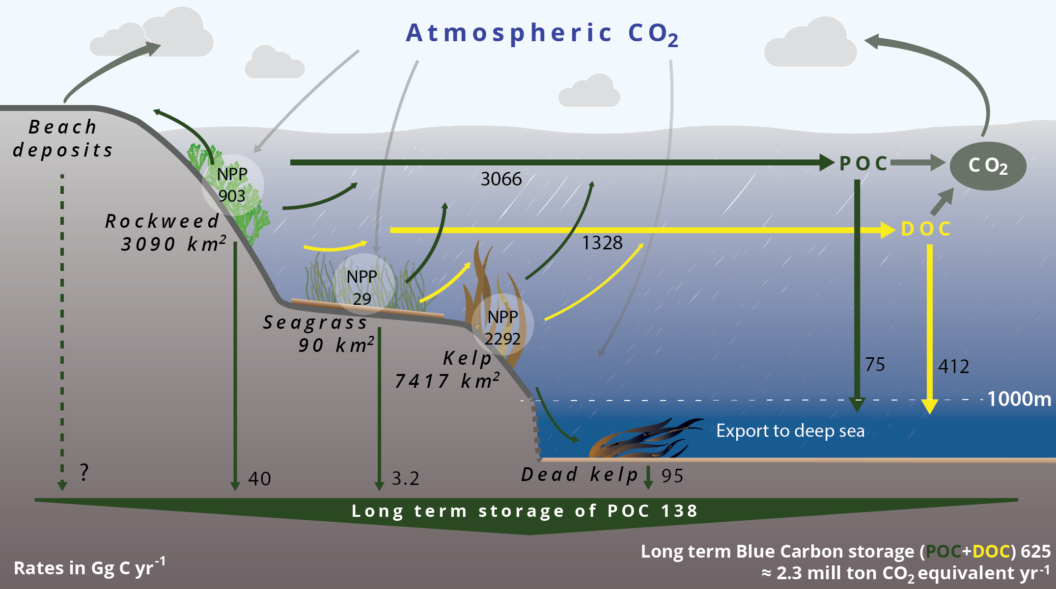
Figure 29. Norwegian blue carbon budget including the kelp forest, rockweed bed, and seagrass meadow habitats. Area extent, rates of net primary production (NPP), export rates, and sequestration of particulate organic carbon (POC) and dissolved organic carbon (DOC) are given for each habitat. POC sequestration occurs in sediments at the shelf and in the deep sea (below 1 000 m depth, termed `long term storage'), while DOC sequestration occurs only in the deep sea (below 1 000 m).

Figure 30. Nordic blue carbon budget including the habitats kelp forests, rockweed beds, and seagrass meadows. Area extent, rates of net primary production (NPP), export rates, and sequestration of particulate organic carbon (POC) and dissolved organic carbon (DOC) are given for each habitat. POC sequestration occurs in sediments at the shelf and in the deep sea (below 1 000 m depth, termed `long term storage'), while DOC sequestration occurs only in the deep sea (below 1 000 m). Numbers are in Gg C y-1 (i.e. 1 000 tonne C y-1). The total sequestration is also given in CO2 equivalents (million tonne CO2 equiv. y-1). Data from Table 8 and Appendix B.
Figure 31. The estimated carbon sequestration (Gg C y-1 = 1 000 tonne C y-1) for kelp forests, rockweed beds, and seagrass meadows in Norway (top left) and the Nordic region (top right). Numbers are compared to regional CO2 emission data for Norway (bottom left) and the Nordic countries (bottom right) in percent. Norwegian and Nordic CO2 emissions are 52 and 214 million tonne CO2 equivalents (2018), respectively (UNFCCC, excluding the LULUCF-sector). Carbon sequestration data from Table 8.
Figure 32. Estimated area of Nordic blue forest habitats (top left), the standing stock of living biomass (top right), total organic carbon stored including both living biomass and organic carbon stored in soft sediments below seagrass meadows (bottom left), and total amount of carbon sequestered (long-term stored) for the Nordic region excluding Greenland, for each of the three blue forest habitats. Data from Chapter 1, Table 8 and Table 12.
Blue carbon at the science-policy interface
In this report, we present a blue carbon budget for the Nordic region, including kelp forests, seagrass meadows and rockweed beds. As described above (Table 8 and Figure 30), we estimated the total Nordic carbon sequestration (long-term storage) for the compiled blue forest habitats at 1 087 Gg C y-1 (equal to 3.9 million tonne CO2 equivalents y-1). This represents the estimate for carbon permanently removed (on climatically relevant time scales) from the biosphere each year by kelp forests, eelgrass meadows and rockweed beds in the Nordic region, and thereby the ability of these blue forest habitats to act as natural carbon sinks. In comparison, the organic carbon stored in living biomass of blue forests was approximately 10 times higher and estimated at 9 236 Gg C y-1 (equal to 33.2 million tonne CO2 equivalents per year). The carbon fluxes of the Nordic blue carbon budget are significant on a national and Nordic scale, with the sequestration of blue carbon in the Nordic region corresponding to around 1.8% of total annual Nordic emissions. For Norway, blue forest carbon sequestration corresponded to around 4.5% of the total annual Norwegian emissions (excluding the LULUCF sector, source: UNFCC, see Figure 31).
The estimated rates in the Nordic carbon budget represent the natural process of carbon uptake and storage in these coastal vegetated ecosystems and are important for the marine carbon cycle and the global climate system. However, for these natural ocean processes to be part of the mitigation options, relevant policy interventions are needed that can manage these natural fluxes of carbon. In the IPCC Special Report on the Ocean and the Cryosphere (SROCC; 2019), two possible management approaches are identified: “First, actions to maintain the integrity of natural carbon stores, thereby decreasing their potential release of greenhouse gases, whether caused by human or climate-drivers; and second, through actions that enhance the long-term (century-scale) removal of greenhouse gases from the atmosphere by marine systems, primarily by biological means”.
The SROCC (2019) includes a synthesis of global estimates for the potential additional sequestration that can be achieved by cost-effective coastal blue carbon restoration at around 0.05 Gt C y–1, which was around 0.5% of the current net anthropogenic emissions from all sources of 10.0 Gt C yr–1. This represents the global potential for policy-based climate change mitigation interventions to restore degraded coastal vegetated habitats, according to the definitions of cost-effectiveness used in the study. It is further noted that improved protection and management can reduce carbon emissions from coastal vegetated ecosystems, thereby decreasing the amount of human-driven and climate-driven greenhouse gases released from these ecosystems if they were degraded or lost. The report entitled “The Oceans as a solution to Climate Change”, from the High Level Panel for a Sustainable Ocean Economy (Hoegh-Guldberg et al., 2019), estimates that increasing the protection and restoration of blue carbon ecosystems (mangroves, seagrasses and salt marshes) could prevent approximately 1 Gt of CO2 from entering the atmosphere by 2050.
In the Nordic region, there have been large reductions in the area distribution of several blue forest habitats in recent decades (Christie & Moy, 2012; Boström et al., 2014; Rinne & Salovius-Laurén, 2020). These habitats are also at high risk from climate change and other human impacts, ranging from the effects of marine heat waves and increased frequency and intensity of storm events, eutrophication, coastal development and habitat fragmentation. This report delivers the first step towards providing a scientific basis for calculating mitigation potentials for the Nordic region either by restoring lost habitats or protecting existing habitats from degradation. Effects of climate change and other human pressures and possible management measures are further described in Chapter 4.
In addition to blue forest habitats, it is also important to identify and conserve the carbon sink areas in the bottom sediments on the coastal shelf, which for the northwestern European shelf has been shown to be considerable (Legge et al., 2020). The impacts of bottom trawling on these benthic carbon stocks are highly uncertain, however the practice is currently widespread and represents one of the few impacts on carbons stocks in marine sediments that is directly manageable.
The fluxes of blue carbon are not included in the national greenhouse gas inventories, and therefore any potential mitigation actions as described above would not be included in national inventory reporting. However, this project has delivered the first step towards providing a scientific basis for how this could be done should Nordic policymakers choose to report voluntarily on blue carbon. There are still considerable knowledge gaps that need to be addressed to reduce the uncertainties in the Nordic blue carbon budget and to report on these fluxes. The IPCC has developed guidelines for the voluntary reporting of mangroves, seagrass and saltmarshes (IPCC Wetlands supplement), however kelp was not included. This would require a follow-up project, with close collaboration between natural scientists and policymakers on how the carbon budget could be operationalized into a national inventory system for greenhouse gases. In the High-Level Panel for a Sustainable Ocean Economy (Hoegh-Guldberg et al., 2019), adopting a methodology for carbon accounting for mangroves, seagrasses and salt marshes, and developing guidelines for macroalgae, were identified as important policy and research priorities.
As highlighted by the SROCC (2019) and Hoegh-Guldberg et al. (2019), management measures to protect and restore blue forest habitats will have a wide range of societal benefits in addition to climate regulation. The SROCC (2019) states that “there is high confidence that coastal wetlands benefit local fisheries, enhance biodiversity, give storm protection, reduce coastal erosion, improve water quality and support local livelihoods (Costanza et al., 2008; Spalding et al., 2014). Coastal ecosystems may keep pace with sufficiently gradual sea level rise, and may be more cost-effective in flood protection than hard infrastructure like seawalls (Temmerman et al., 2013; Möller, 2019)”. Protection and restoration of blue forest habitats (including mangroves) is therefore identified as a “no-regret” mitigation option, which offers a combination of carbon mitigation with broader societal and environmental co-benefits.
The Nordic Ministerial Declaration on Oceans and Climate (2019) lays out the ambitions for increased Nordic collaboration on several areas that are highly relevant and compatible with the key findings and policy recommendations from the Nordic Blue Carbon Project, especially the following key points:
- Increase the resilience of Nordic sea areas to climate change, through ecosystem-based management of human activities impacting the seas, and by supporting the development of ecologically coherent and well-managed networks of marine protected areas and other area-based management measures.
- Encourage and strengthen scientific research that will enable us to identify and maintain natural ocean carbon sinks in Nordic sea areas.
Conclusions
In this chapter, areal coverage (WP1) and production and sequestration rates (WP2) for Nordic blue carbon ecosystems were merged with compiled data from the scientific literature to inform an updated overview of carbon cycling in blue forests and provide an up-to-date Nordic blue carbon budget.
For Norway, the largest contributor to blue forest carbon sequestration was kelp forest, with an estimated sequestration rate of 1.8 million tonne CO2 equivalents per year (503 000 tonne C y-1), representing the large areas covered by kelp forest along the Norwegian coast. For comparison, Norwegian kelp forest carbon sequestration corresponded to around 3.6% of the total Norwegian CO2 emissions to the atmosphere (52 million tonne CO2 equivalents, excluding LULUCF). For the entire Nordic region, the kelp forest carbon sequestration was estimated at 2.7 million tonne CO2 equivalents per year (746 000 tonne C y-1).
Carbon sequestration from rockweed beds was estimated at 0.4 and 0.8 million tonne CO2 equivalents per year for Norway and the Nordic region, respectively, corresponding to 117 000 and 209 000 tonne C y-1.
Carbon sequestration from seagrass meadow was estimated at 0.02 and 0.5 million tonne CO2 equivalents per year for Norway and the Nordic region, respectively, corresponding to 4 600 and 133 000 tonne C y-1.
Including all the Nordic countries (excluding Greenland), we estimated the blue forest carbon sequestration to be 3.9 million tonne CO2 equivalents per year (1.1 million tonne C y-1). This corresponds to ~1.8% of the Nordic CO2 emissions annually (214 million tonne y-1 in 2018, excluding LULUCF). These data exclude estimates for Greenland because predicted blue forest areas for Greenland are highly uncertain.
Key uncertainties in these estimates are the export and fate of DOC production from kelp, rockweed and seagrass, and the transport and sequestration rates of particulate organic carbon (POC) in shelf and deep-sea systems. The findings in this report highlight the importance of Nordic blue forest habitats and their significant contribution to carbon sequestration in shelf and deep-sea habitats.
Chapter 4 – Blue forests now and in the fu|ture: pre|ssures and manage|ment
Environmental change impacts organisms in several ways. Changes can impact on organisms directly, causing physiological and/or behavioral responses that are either harmful or beneficial to the organism. These responses are likely to also include alterations in the organism’s interactions with the rest of the ecological system, thus affecting larger parts of the system indirectly (see Appendix C for a comprehensive list of references). Seemingly small impacts directly affecting one group of organisms can in fact trigger a cascade of effects and potentially cause major structural changes that alter the stability of the entire ecological system (e.g. Pinnegar et al., 2000). Alas, species that do not respond directly to ongoing environmental changes can still be severely impacted, because the stability of the ecosystems on which they depend is compromised. Although a great deal of work has been carried out with regards to single species’ responses to climate change, including distribution predictions, system response studies and predictions are less common (but see for instance Stige et al., 2010; Griffith et al., 2018; Kotta et al., 2019).
In this work package, we aim to broaden the view of the general ecological relationships governing the stability of Nordic blue forests today, and in turn contribute to the understanding of how different pressures related to climate change may alter these relationships and thereby drive change in the ecological systems over time. Lastly, the aim has been to establish whether management efforts have the potential to mitigate the negative impacts, and to identify which measures are likely to be the most effective.
To better understand how pressures and their effects on all the different ecological relationships culminate in system responses in Nordic blue forests, we have plugged present day qualitative knowledge about species’ interactions and pressure responses into a novel network simulation framework. This simulation framework facilitates further quantitative analyses that yield semi-quantitative results, which are useful in pinpointing which ecological relationships are likely to be the most important for maintaining system structure and stability. Pinpointing these relationships gives way to more accurate targeting of potential management efforts to increase system resilience, which will be particularly important in environments of rapid change. The framework also allows for simulations of additional pressures, for instance applying pressures consistent with future climate scenarios and pressures representing potential mitigating efforts.
The simulations thus facilitate relative comparisons of characteristics important for stability in different system types (e.g. kelp forests, seagrass meadows and rockweed ecosystems), as well as holistic evaluations of which suit of management efforts is likely to be the most effective in safeguarding blue forests for the future.
Methods
A knowledge base was built using Parsifal, an online literature review tool. A total of 924 papers were imported, the only criteria being that they were ecological studies concerned with either kelp forests, seagrass meadows or rockweed ecosystems. Most of the work was carried out in 2017 and 2018, and papers that have been published since may not have been included due to limited resources and work capacity. In the filtering process, we focused on papers that were studying or reviewing ecological relationships in Nordic countries, and that had clear descriptions of the nature of these relationships. The result was approximately 30 papers (see Appendix C), which were used as the basis for discussions with the work group (mostly NVIA-based experts), from which schematic presentations of the ecological networks were drawn using the free and open source Dia software (Phase 1 in Figure 33, also see example in Figure 33). These presentations were imported directly into R, and formed the basis of the qualitative network analyses that were performed using a combination of the QPress (Melbourne-Thomas et al., 2012) and the RandomForest (Liaw & Wiener, 2012) packages in R. Most of the data handling and graphical displays were executed using the tidyverse package (Wickham et al., 2019) and ggplot2 extensions (like patchwork; Pedersen, 2020).
Using QPress, a vast number of interaction matrices were simulated, all with the same qualitative properties as the schematic Dia graphs, meaning that all positive interactions were assigned values (weights) ranging from small negative to large positive (1 being the largest), and all negative interactions were assigned values ranging from large negative (-1) to small positive (Phase 2 in Figure 33). The community matrix was then tested for stability. A stable matrix is one where the balance between the different components in the network, given the symphony of interactions between them, does not change over time. In other words, for a system to be considered stable, the result of all interactions must ensure the continued presence of all its components (Phase 3 in Figure 33). By this definition, a stable kelp forest for instance, must be able to retain both urchins and kelp, in balance. For every system, simulations were run until 10 000 stable matrices were obtained (usually amounting to over 100 000 unstable ones). The properties of the stable and unstable networks, and what separates the two, were then investigated using random forest analyses (Phase 4 in Figure 33).
The environment is now rapidly changing, and a multitude of important questions naturally follows: What happens to the stability and structure of the ecosystems when subjected to these environmental changes? For instance, what is likely to happen to the Norwegian seagrass meadows if sea temperatures along the coastline increase? The meadows are likely to change, but how and by what mechanisms? And can anything be done to mediate possible detrimental impacts? Furthermore, what happens when multiple pressures are applied at the same time, for instance temperature increase, eutrophication, overfishing, light reductions and sedimentation? Questions like these are very difficult to answer using a purely quantitative approach, because we most often do not know the exact properties of the different interactions in the ecological systems or exactly how pressures from the outside affect them. Bringing these questions into a simplified simulation framework, in which a vast number of possibilities can be tested, gives us an idea of how these systems are most likely to work, and what the most likely outcomes of changed pressures are (Phase 4 in Figure 33). Provided that the network descriptions serving as inputs have captured the nature of the most important ecological relationships, the outputs can be very useful in planning and prioritizing the management efforts.
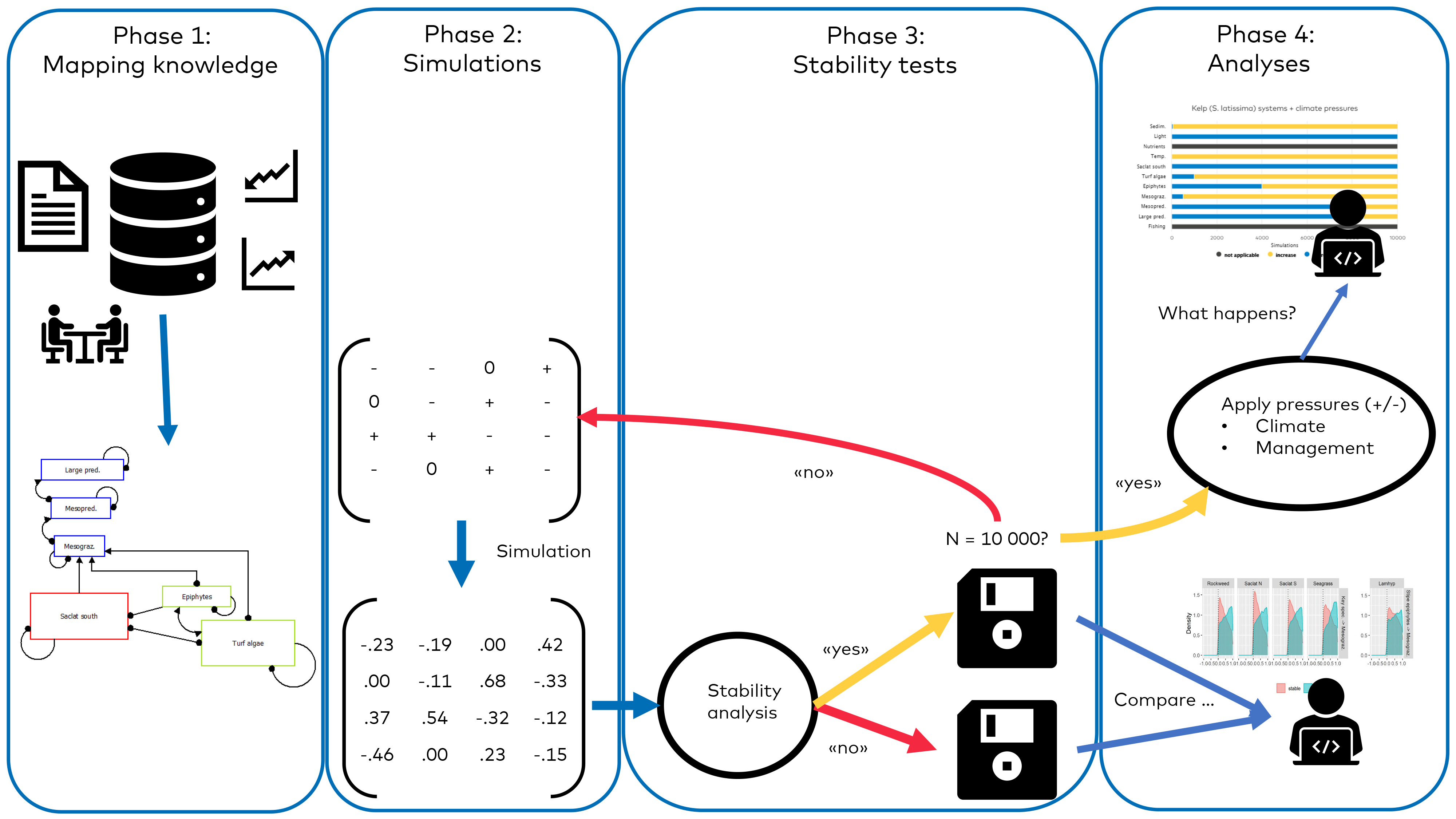
Figure 33. Schematic presentation of general approach in WP4: Phase 1 comprises a general literature search and review, as well as discussions with the expert group to form an overview of qualitative knowledge describing the most important ecological relationships, as well as impacts of environmental change in the different ecosystems. In Phases 2 and 3, the assembly of quantitative knowledge is used to form a simulation framework, which yields results on which quantitative tests and analyses can be run in Phase 4.
Results and discussion
Ecological interactions in Nordic blue forest ecosystems
Based on the literature review and discussions within the project, we decided to create five representations of Nordic blue forest ecosystems. These correspond to the four ecosystems discussed, particularly in Chapter 1, but with two representations of sugar kelp forests. The rationale behind this division is the difference in negative impacts of urchin grazing. While northern populations are subjected to severe urchin grazing, the southern populations generally are not (see e.g. Rinde et al., 2014). The five representations formed the basis on which we could run simulations, the results of which were analyzed using quantitative methods. The networks present the most important interactions in
- Tangle kelp (Laminaria hyperborea) kelp forests
- Northern sugar kelp (Saccharina latissima) kelp forests (strong influence of urchins)
- Southern sugar kelp (Saccharina latissima) kelp forests (urchins are lumped together with other mesograzers)
- Seagrass meadows (focused on Zostera marina meadows)
- Rockweed ecosystems (multitude of foundation species, mainly in the order of Fucales)
There are some notable differences between the different systems with regards to functional groups (Table 10). For instance, epiphyte communities in tangle kelp forests are divided into two groups 1) epiphytes growing on the kelp stipes and 2) epiphytes growing on the kelp blades. These groups, although both epiphytic, have completely different ecological roles. The epiphyte communities found on the stipes are an important part of the kelp forest understory vegetation. Many of these are perennial species with a bushy or leafy morphology that provide shelter, nursery and feeding grounds for a myriad of smaller animals (see for instance Norderhaug & Christie, 2011). A diverse and voluminous community of stipe epiphytes is usually a sign of a successionally mature tangle kelp forest. Sugar kelp (S. latissima) has a completely different morphology, with much thinner and shorter stipes, that is much less suitable as substrate for these epiphytes. Hence, in the sugar kelp systems as well as in seagrass and rockweed systems, the stipe epiphytes are lacking as a functional group. The epiphytes found on tangle kelp blades, on the other hand, resemble epiphyte communities found on the blades of sugar kelp (and on rockweed and to some extent on seagrass). These are predominantly opportunistic species that are more likely to overgrow the macrophyte and cause harm (Andersen et al., 2019). The opportunistic epiphyte communities are actually very similar to the turf communities that partly outcompete kelp in many areas of the world (Filbee-Dexter & Wernberg, 2018), and it is therefore reasonable to assume that a positive feedback mechanism is present between the epiphyte communities and the turf communities.
The animal functional groups, i.e. large predators, mesopredators and mesograzers, largely consist of the same groups of organisms, but often different species depending on ecosystem and geography. For instance, in the functional group called large predators, cod is probably the most important species in the wave exposed areas, where typically kelp forests are found. The notion that wolffish may also have been historically important in Nordic kelp ecosystems has gained support recently, but these populations are currently generally small (Norderhaug et al., 2020). Anadromous salmonids, like sea trout which mostly stay and graze in fjord areas in their marine life stages, may be particularly significant predators in rockweed and seagrass areas close to salmonid rivers. Among mesopredators, the smaller predators in the ecosystems mostly foraging on grazers, crustaceans like brown crab, king crab, lobsters, and fish like wrasses and gobies are notable examples. Among the mesograzers, there are diverse communities of small crustaceans, echinoderms and gastropods, with species compositions also varying both geographically and among the different systems. For a full list of references used to evaluate the ecological relationships and roles, see Appendix C.
Table 10. Mapping of the most important interactions in five representations of Nordic blue forest ecosystems, based on documentation and evaluation by the working group. For simplicity in comparing the systems, epiphytes growing on blades are denoted as Epiphytes, while stipe epiphytes (essentially only present in tangle kelp forests) are specified as Stipe epiphytes. The symbols -* and -> indicate negative and positive interactions respectively (also given in the Effect column). For references, see Appendix C.
| Interaction | Effect | N. sugar kelp | S. sugar kelp | Tangle kelp | Seagrass | Rockweed |
| Large pred. -* Mesopred. | Negative | X | X | X | X | X |
| Mesopred. -* Mesograz. | Negative | X | X | X | X | X |
| Mesograz. -* Epiphytes | Negative | X | X | X | X | X |
| Mesograz. -* Turf algae | Negative | X | X | X | X | X |
| Turf algae -* Key spec. | Negative | X | X | X | X | X |
| Epiphytes -* Key spec. | Negative | X | X | X | X | X |
| Turf algae -* Turf algae | Negative | X | X | X | X | X |
| Epiphytes -* Epiphytes | Negative | X | X | X | X | X |
| Key spec. -* Key spec. | Negative | X | X | X | X | X |
| Large pred. -* Large pred. | Negative | X | X | X | X | X |
| Mesopred. -* Mesopred. | Negative | X | X | X | X | X |
| Mesograz. -* Mesograz. | Negative | X | X | X | X | X |
| Epiphytes -> Turf algae | Positive | X | X | X | X | X |
| Urchins -* Key spec. | Negative | X | X | |||
| Mesopred. -* Urchins | Negative | X | X | |||
| Urchins -* Urchins | Negative | X | X | |||
| Key spec. -> Mesograz. | Positive | X | X | X | X | |
| Key spec. -> Mesopred. | Positive | X | X | X | X | X |
| Mesopred. -> Large pred. | Positive | X | X | X | X | X |
| Mesograz. -> Mesopred. | Positive | X | X | X | X | X |
| Epiphytes -> Mesograz. | Positive | X | X | X | X | X |
| Turf algae -> Mesograz. | Positive | X | X | X | X | X |
| Key spec. -* Turf algae | Negative | X | X | X | X | |
| Turf algae -> Epiphytes | Positive | X | X | X | X | X |
| Urchins -> Mesopred. | Positive | X | X | |||
| Mesograz. -* Stipe epiphytes | Negative | X | ||||
| Stipe epiphytes -* Stipe epiphytes | Negative | X | ||||
| Key spec. -> Stipe epiphytes | Positive | X | ||||
| Key spec. -> Large pred. | Positive | X | ||||
| Stipe epiphytes -> Urchins | Positive | X | ||||
| Stipe epiphytes -> Mesograz. | Positive | X | ||||
| Urchins -* Stipe epiphytes | Negative | X | ||||
| Mesograz. -* Key spec. | Negative | X |
Extensive and detrimental urchin grazing on macrophytes is predominantly reported as a problem in tangle kelp and northern sugar kelp forests (Rinde et al., 2014), which is why urchins are given special emphasis by separating them from the general mesograzer box in these systems. Urchins are of particular interest, because urchin density control is a much discussed and highly relevant target for trying to restore and rebuild kelp forests today (Wallhead et al., 2018).
Although the remaining defined groups (large predators, mesopredators and mesograzers) comprise different species depending on the system type (kelp, seagrass or rockweed) and geography, they do encompass similar functions (Table 10 and Figure 34).
Figure 34 displays the network representing the tangle kelp (Laminaria hyperborea) forest systems and contains both internal interactions and external pressures that were deemed the most important based on the literature review and discussions in several workshops and meetings. See Appendix C for a full list of literature references.
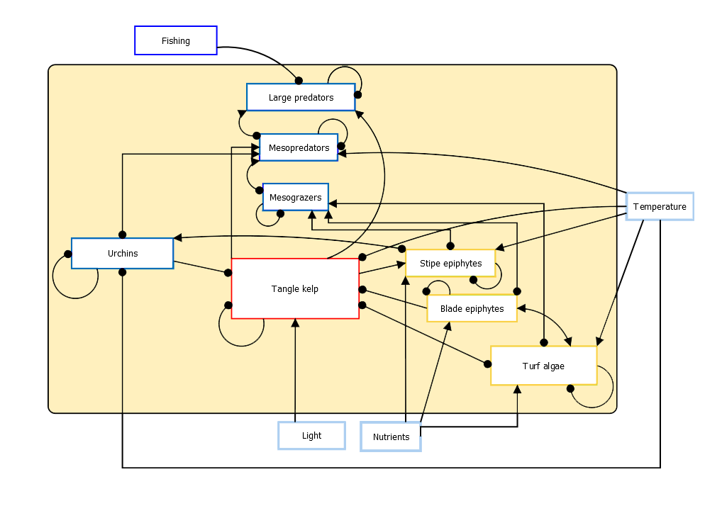
Figure 34. Schematic presentation (Dia graph) of a simplified web of interactions in tangle kelp (Laminaria hyperborea) forest systems. The shaded green box comprises internal interactions between components within the ecological system, while components outside the yellow box (i.e. temp, light, nutrients and fishing) are considered external pressures that are acting from outside of the ecological system. Positive and negative interactions are indicated by arrowheads and bullets respectively. All biological components will naturally be subjected to some degree of self-limiting, hence the “boomeranging” bullets. Blue boxes contain animal groups acting on the kelp through top-down interactions, while the yellow boxes contain groups mainly comprised of algae, that either depend on or compete with the kelp. The light blue boxes contain environmental pressure variables.
Interactions that influence the stability of Nordic blue forest ecosystems
There are several similarities in the way the Nordic blue forest systems seem to be organized (see references in Appendix C), and thus the results with regards to both stability properties and pressure responses are similar in many ways. The simulation results with regards to stability were analyzed using random forest analyses, the results of which are summarized across all systems in Figure 35.
The most defining interactions found in stable systems of all types involved turf algae, epiphytes and mesograzers. A strong impact of turfs and epiphytes on the main macrophyte (kelp, seagrass or rockweed) did in most cases lead to unstable communities. At the same time, the presence of mesograzers was shown as particularly important for securing the stability of most of the simulated systems. Stable systems generally had strong links between mesograzers and the turf and blade epiphyte communities, indicating that boosting mechanisms leading to increased grazing intensities (i.e. mesograzer population increase) following increases in both blade epiphyte and turf communities are important for system stability (Figure 36). The results also highlight the importance of mesograzer communities being able to remain in the systems independently of fluctuations in the key species (or in the case of tangle kelp systems, the stipe epiphytes) (Figure 37). In other words, the mesograzers’ ability to interfere with the competitive relationship between turf algae and forest forming species (seagrass, kelp and rockweed) was identified as one of the most important properties of stable blue forest systems. A strong presence of mesograzers in all these systems thus seems crucial for maintaining a healthy blue forest system over time.
The influence of urchin populations on kelp populations (northern sugar kelp and tangle kelp) also separated stable from unstable communities. In most of the simulations that were stable, the influence of urchins on kelp was in the intermediate to low range, with few at the extremely low end. We know that many kelp forest areas along the coast of Norway are changing due to increases or relief in the pressure from urchins (Rinde et al., 2014), and our results indicate that reducing (and not completely removing) this pressure may help the kelp regain the ground in areas where it is currently largely disappearing. Completely removing internal negative pressures from a system, such as complete removal of urchins, may prove ineffective in the long term. Systems including a certain amount of internal negative pressure on the habitat-forming species are more likely to also have robust mechanisms controlling for these pressures. For instance, top-down control of destructive grazers such as urchins may disappear if urchins completely vanish from the kelp forest systems for longer periods. Complete removal of internal negative pressure may thus lead to lower resilience against fluctuations in the negative pressures later on, for instance lower resilience in kelp forests towards pulse increases in urchin populations.
All in all, the simulations suggest that management measures aimed at securing robust mesograzer communities, and efforts to reduce the negative pressure from urchins are likely to be the most effective in securing the stability of blue forest systems today. Stable systems are generally more robust when subjected to new pressures, which is particularly important in the face of climate change. Understanding and securing system stability should therefore be the top priority in the management of blue forest systems. The measures best suited to securing a healthy mesograzer presence are still largely an open question in need of more research. Potential measures could entail, for instance, providing temporary mesograzer refuges by establishing artificial reefs/structures that can be utilized when the key species and the habitat are struggling.
To begin mapping out which management strategies are likely to be the most effective in mitigating negative impacts from outside the systems, external pressures were added to the system simulations (Phase 4 in Figure 33). These pressures can then be increased or released, simulating both environmental change (e.g. increased temperature) and management efforts (e.g. reductions in nutrient loads or controls on fisheries). However, in doing so we introduce new uncertainties into the system simulations, and caution therefore needs to be applied when interpreting these simulations.
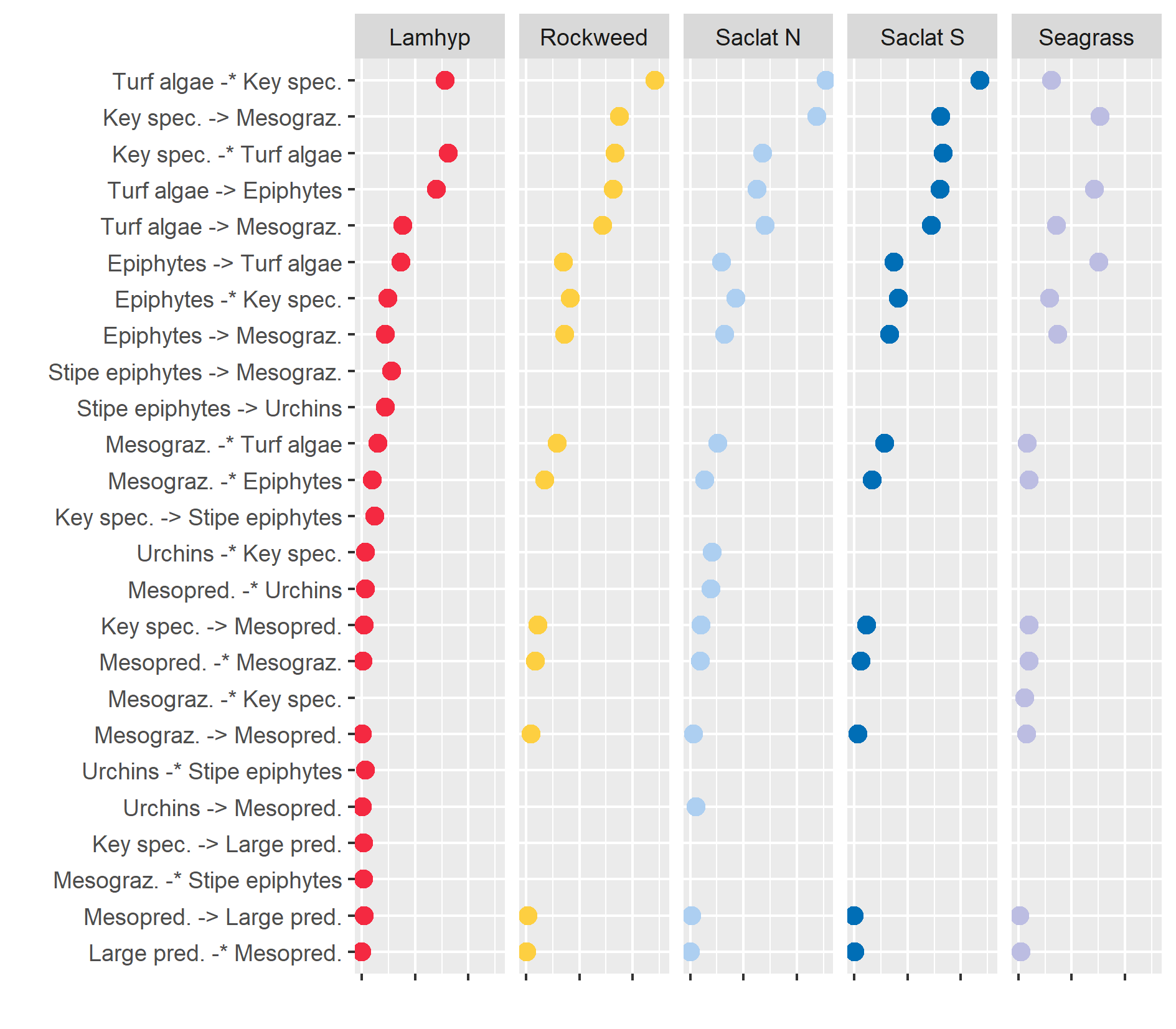
Figure 35. Output from the random forest analyses of simulation results for each of the five system types; tangle kelp = Lamhyp, Saclat N = northern sugar kelp, Saclat S = southern sugar kelp. The symbols -* and -> indicate negative and positive interactions respectively. Placement of dots along the x-axis indicates the relative importance of the specific nature of the given interaction (whether the interaction is strong or weak), in defining stability. Thus, the x-axis Left – Right placement is equal to Low – High relative importance.
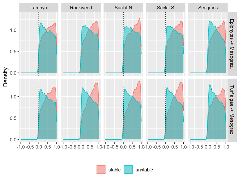
Figure 36. Density plots of simulated interaction weights (x-axis) in stable vs. unstable communities. -1 is strong negative, while +1 is strong positive. The peaks indicate in what range of values the frequency of stable or unstable communities were the highest and shows that stability is most often acquired when the mesograzer population is strongly and positively impacted by increases in turfs and epiphytes. Mesograzers will thus respond quickly to fluctuations in turf and epiphyte communities in most of the stable systems.
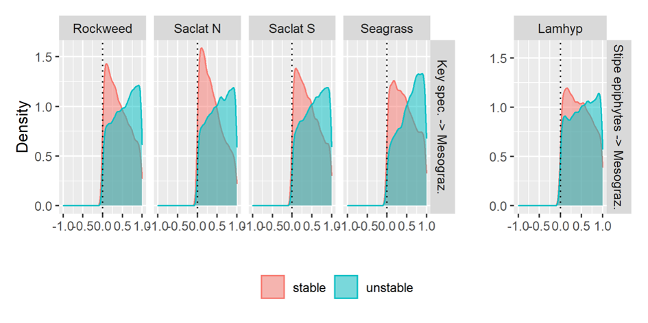
Figure 37. Density plots of simulated interaction weights (x-axis) in stable vs. unstable communities. -1 is strong negative, while +1 is strong positive. The peaks indicate in what range the frequency of stable or unstable communities were the highest, and shows that stability is most often acquired when the link between mesograzers and the key species is weak. Mesograzers will thus respond slowly to fluctuations in the key species in most of the stable systems.
Environmental change and responses to pressures in Nordic blue forest
The report “Climate in Norway 2100” presents past, present and future projections for climate in Norway (Hanssen-Bauer et al., 2015; Hanssen-Bauer et al., 2017), and the selection and direction of climate change drivers in this project were based mainly on this work. Climate change is expected to drive the ocean climate in Nordic areas towards warmer and more acidic water masses. Increases in riverine and landmass run-off are also expected, which will contribute to increased concentrations of organic matter (both dissolved and particulate) in coastal water masses, with possible consequences being coastal water darkening and increased sedimentation in coastal areas (Aksnes et al., 2009; Frigstad et al., 2013; de Wit et al., 2016). Other anthropogenic pressures, such as overfishing and eutrophication, will act as additional pressures on the blue forests systems.
The different blue forest systems are expected to be affected by the different climate pressures in different ways, largely because they inhabit different niches (see references listed in Appendix C). The tangle kelp (Laminaria hyperborea) generally occupies hard-bottom areas subjected to a fair amount of water movement from either currents or waves, while the sugar kelp (Saccharina latissima) is generally found in more sheltered hard-bottom areas. Rockweeds are found in both exposed and sheltered hard-bottom areas, but at shallower depths than the kelps, while seagrasses are found in soft-bottom areas. Changes in water temperature, light availability and sedimentation are certainly expected to vary in magnitude among these different parts of the environmental space. For instance, sedimentation is expected to change very little in hard-bottom areas, where water movement is high and particles are constantly flushed out. More sheltered hard-bottom and soft-bottom areas, where particles linger to a greater extent, are expected to experience increased sedimentation rates due to increased particle loadings. Similarly, the effect of coastal darkening will be more severe in deeper layers, because more light is absorbed and scattered by organic matter concentrations as light travels through the water column. Hence, tangle kelp is less likely to be impacted by a general increase in sedimentation rates compared to, for instance, seagrasses, while rockweeds are less likely to be impacted by coastal darkening than, for instance, sugar kelp. There are therefore some clear differences in how climate change is portrayed in the different system simulations, and consequently how environmental pressures impact the different system simulations. There are also some changes for which there was insufficient knowledge in 2018 to qualitatively assign effects on the system, and which were therefore omitted from the simulations. This is particularly pertinent to changes in pH, where effects on most groups, including macrophytes, are still unclear (Gao et al., 2019). Ice scouring is another difficult potential pressure, because changes in ice cover along the coastline due to climate change is highly variable. For instance, some areas are likely to experience more scouring due to reductions in ice thickness and thereby less stable ice covers, while other areas are likely to experience less scouring due a general disappearance of ice cover all together. In any case, scouring is predominantly assumed to affect rockweeds.
For all blue forest systems, the following climate change pressures were added to the simulations (see Table 11 and example for southern sugar kelp in Figure 38): increased temperature and sedimentation, and reduced light. For most of the simulations there was a negative response in the key macrophyte to the addition of climate change pressures (Table 11). The abundance of rockweed, seagrass and southern sugar kelp were reduced in all simulations. Sugar kelp in the north, as well as tangle kelp, did however increase in a minor part of the simulations (~ 10–15%). When climate change was assumed to cause a relief of ice scouring, rockweeds increased in some simulations as well (> 20%).
Climate change pressures led to an increase in turf algae abundance in most of the simulations (> 80% of kelp and rockweed simulations, > 70% of seagrass simulations) (see response plot for sugar kelp systems in Figure 38, and Appendix C for responses in the four other systems). Epiphytes increased in most of the southern sugar kelp (~ 60%), rockweed (~ 65%) and seagrass (~ 75%) pressure simulations, while decreasing in almost half of the northern sugar kelp (S. latissima) and tangle kelp (L. hyperborea) simulations. In general, an increase in turf algae and blade epiphytes will act to destabilize the blue forest systems, which will further reduce the resilience against the negative pressures from climate change.
Mesograzers generally increased in abundance in most simulations, mostly due to the boosting effect of increases in epiphyte and turf abundances. Mesopredators in the tangle kelp (L. hyperborea) systems increased in the majority of the pressure simulations (a little over 60%), while the pressure mostly led to a decrease of this group in the other blue forest systems (~ 70% of northern sugar kelp (S. latissima), ~ 85% of southern sugar kelp and rockweed, and over 95% of the seagrass simulations). Large predatory fish were reduced in the same amount of simulations as mesopredators, except in the tangle kelp simulations, where the number was higher (reductions in 75% of the simulations).
Figure 38. Example: Pressure responses in the southern sugar kelp (Saccharina latissima) forest systems, when exposed to climate change (increases in temperature and sedimentation and reductions in light).
In addition to the effects of climate change on the blue forest systems, we added other anthropogenic pressures, such as increase in nutrient loading (i.e. eutrophication) and increased fishing (i.e. overfishing). Overall, these additional pressures had only minor effects on the simulation results with respect to abundance of the key species (kelp, rockweed or seagrass) in all the blue forest systems (see example for southern sugar kelp in Figure 39 and Appendix C for the four other blue forest system types). These effects were mostly seen in other species groups, which implies further shifts in structure and functioning of the ecological system, which is likely to render system recovery even more difficult. Furthermore, simulations including eutrophication or overfishing as single pressures did in fact show negative effects on the key species in the vast majority of simulations. This means that continued efforts to limit eutrophication and overfishing are crucial for protecting kelp, rockweed and seagrass populations.
Figure 39. Example: Pressure responses in the southern sugar kelp (Saccharina latissima) forest systems, when exposed to climate change, overfishing and eutrophication.
Possible management measures to safeguard blue forests in the future
While securing the stability of blue forest systems today is probably the most important measure for improving system resilience and safeguarding blue forests for the future, our simulations suggest that further measures may mitigate some of the detrimental impacts of climate change on the key species.
Improved light condition was the most effective single-action measure for improving the resilience of kelp and rockweed in the pressure simulations (see response plot for sugar kelp systems in Figure 40 and Figure 41 and Appendix C for responses in the four other blue forest systems). In contrast, reductions in fishing pressure and nutrient loadings were the most effective single-actions for improving the resilience of seagrass.
A full range of actions, targeting nutrient loadings, sedimentation and light conditions, as well as reductions in fishing pressure, were substantially more efficient in improving conditions for the key species in all systems (see Table 11).
Table 11. Summary of the pressure simulation results with regards to the key species tangle kelp (Laminaria hyperborea), sugar kelp (Saccharina latissima), rockweed or seagrass. The sugar kelp is divided into northern and southern populations, because sea urchin grazing is a dominant negative pressure on the kelp only in the northern regions (see e.g. Rinde et al., 2014). The percentages refer to relative amounts of simulations in which either a negative or a positive response in the species occurred.
| System pressure simulations | ||||||||||
| Tangle kelp | Rockweed | Sugar kelp N | Sugar kelp S | Seagrass | ||||||
| Response category | Pos | Neg | Pos | Neg | Pos | Neg | Pos | Neg | Pos | Neg |
| Climate change (temp + sedim + light) | 15% | 85% | 0% | 100% | 10% | 90% | 0% | 100% | 0% | 100% |
| Mitigating measures | ||||||||||
| Targeting nutrients | 30% | 70% | 0% | 100% | 10% | 90% | 15% | 85% | 25% | 75% |
| Targeting light | 60% | 40% | 20% | 80% | 50% | 50% | 25% | 75% | 5% | 95% |
| Targeting sedimentation | - | - | 5% | 95% | 25% | 75% | 5% | 95% | 10% | 90% |
| Urchin control | 30% | 70% | - | - | 25% | 75% | - | - | - | - |
| Reducing fishing pressure | 15% | 85% | 5% | 95% | 15% | 85% | 10% | 90% | 15% | 85% |
| Full range (all measures above) | 80% | 20% | 75% | 25% | 80% | 20% | 70% | 30% | 35% | 65% |
Figure 40. Example: Pressure responses in southern sugar kelp (Saccharina latissima) forest systems, when exposed to climate change, but improved light conditions as single-action management measure.
Figure 41. Example: Pressure responses in southern sugar kelp (Saccharina latissima) forest systems, when exposed to climate change, and a full range of management measures.
Comprehensive work has already been undertaken to detail concrete management strategies, particularly for sugar kelp forests and seagrass meadows in Norway. These include a full range of specific targets and measures, also specified for different industries, sectors and river basin districts (vannregioner). Several of the suggested strategies target the key pressures we have identified, and are thus likely to positively impact all blue forest systems and be highly relevant in a broader Nordic context:
- Vurdering av tiltak mot bortfall av sukkertare (English: Assessment of management measures against loss of sugar kelpS. latissima.) Arbeidsgruppen for sukkertare. Rapport for Klima- og Forurensningsdirektoratet. Rapport TA 2585. 2009
- Tiltak for å ta vare på truet natur: Kunnskapsgrunnlag for 90 truete arter og 33 truete naturtyper. (English: Actions to conserve threatened nature: Knowledge bases for 90 threatened species and 33 threatened nature types) NINA Rapport 1646. Norsk institutt for naturforskning. 2019.
It is very important to note that the probability of successfully mitigating climate impacts is likely to increase if measures aimed at securing the stability of the systems are prioritized. Securing functional mesograzer communities and exerting urchin control seem particularly important in this respect. The effect of habitat fragmentation and destruction due to changes in land/sea use is not tested nor discussed in the present project, but is generally considered to be one of the most serious threats to the stability of the earth’s ecosystems and biodiversity (see e.g. IPBES Global assessment report on Biodiversity and Ecosystem services, 2019). Minimizing further fragmentation of blue forests and improving connectivity in areas where that is possible, for instance by establishing strategic MPAs and enforcing strict regulations with regards to alterations of landscape in the coastal zone, are also likely to be effective stabilizing measures.
Conclusions
In this chapter, we used qualitative knowledge of the ecology of the blue forest systems to build five different network simulation frameworks. This provided insight into the ecological relationships that are most important in maintaining blue forest system structure and stability, and allowed for investigations of climate change impacts and potential mitigation measures. The simulations showed that increases in turfs and blade epiphytes (mostly fast-growing, short lived algae) in most cases acted to destabilize Nordic blue forest systems. The simulations also showed that the increased impact of these groups is likely to be the consequence of climate change (increased temperatures and sedimentation, reduced light availability). However, the mesograzers’ (small grazers that eat plants, like snails, shrimps and amphipods) ability to interfere with the competitive relationship between turfs and forest-forming species (seagrass, kelp and rockweed) was identified as one of the most important properties of stable blue forest systems. This means that facilitating and maintaining a strong presence of mesograzers in all these systems, independent of fluctuations in kelps, rockweed and seagrass populations, is likely to be very effective in increasing the system resilience and mitigating the negative impacts of climate change. More knowledge is however needed to figure out how to effectively achieve this. One possibility may be to establish suitable artificial mesograzer refuges (such as artificial reefs), so that mesograzers are able to persist in areas where their habitat is periodically under pressure, but little is known about what properties these structures should have or their potential effects. In areas impacted by severe urchin grazing (also a mesograzer, but considered separately in the analyses), efforts to reduce but not completely remove the urchin populations were shown to likely increase the blue forest system’s resilience. Our simulations also indicate that the continued efforts to limit additional human impacts is important in safeguarding blue forest systems for the future. To mitigate the effects of climate change, we found that improved light conditions was the most effective target for measures in kelp and rockweed habitats. For seagrass populations, we found that reductions in fishing pressure and nutrient loadings were the most effective mitigating targets. The effect of habitat fragmentation and destruction due to changes in land/sea use is not tested or discussed in the present project, but is generally considered to be one of the most serious threats to the stability of the earth’s ecosystems and biodiversity, which should also be kept in mind in planning for both protection and restoration. It is also important to note that knowledge gaps, for instance with regards to the effect of ocean acidification (not included in the simulations), increase the uncertainty of the analyses. Furthermore, the assessment of how environmental change impacts the functional groups is mostly based on a limited degree of experimental laboratory work, with a limited number of representative species and limited knowledge of current day distribution patterns, which does not necessarily provide a realistic view of species’ tolerance limits in the future, especially given the full range of changes that are happening. Continued work to bridge knowledge gaps, to better understand the mechanisms governing ecosystems, their vulnerabilities and the species they comprise is vital for decreasing these uncertainties and planning for effective ecosystem management now and in the future.
Chapter 5 - Policy recommen|dations
The following text was produced based on presentations and discussions at the final workshop of the Nordic Blue Carbon Project on 21–22 November 2019, gathering scientists, policymakers and stakeholders from Norway, Sweden, Denmark, Finland and the UK. It summarizes the policy recommendations from the project scientists and was distributed by email to relevant Nordic policy institutions and working groups under the Nordic Council of Ministers in December 2019.
Policy Brief on Nordic Blue Carbon
Policy relevance. The profound importance of coastal and marine ecosystems for both climate mitigation and adaptation strategies is highlighted in recent reports, such as the High Level Panel for a Sustainable Ocean Economy[1]High Level Panel for a sustainable Ocean Economy: The Ocean as a Solution for Climate Change: 5 Opportunities for Action https://www.oceanpanel.org/climate and the IPCC Special Report on the Ocean and the Cryosphere[2]IPCC Special Report on the Ocean and Cryosphere in a Changing Climate [H.- O. Pörtner, D.C. Roberts, V. Masson-Delmotte, P. Zhai, M. Tignor, E. Poloczanska, K. Mintenbeck, M. Nicolai, A. Okem, J. Petzold, B. Rama, N. Weyer (eds.)]: https://www.ipcc.ch/srocc/. Further, the recent Nordic Ministerial Declaration on Oceans and Climate[3]Nordic Ministerial Declaration on Oceans and Climate, 30.10.19: https://www.norden.org/en/declaration/nordic-ministerial-declaration-oceans-and-climate extends Nordic marine cooperation to several areas highly relevant for Blue Carbon# habitats, for example “identify and maintain natural ocean carbon sinks” and “supporting the development of ecologically coherent and well managed networks of marine protected areas”.
Norwegian and Nordic Blue Carbon habitats. The Nordic countries combined have 11% of the world’s coastline[4]https://en.wikipedia.org/wiki/List_of_countries_by_length_of_coastline. The area of Norwegian kelp forests[5]Gundersen et al. (2011). CO2 uptake in marine habitats - an investigation. NIVA report no. 6070-2010. 25 pp. (In Norwegian with English summary) is around 8 000 km2 and is known to be among the largest in northern Europe. The Nordic seagrass meadows[6]Boström et al. (2014). Distribution, structure and function of Nordic eelgrass (Zostera marina) ecosystems: implications for coastal management and conservation. Aquatic Conserv: Mar. Freshw. Ecosyst.24: 410–434 cover some 2 000 km2 and some of the meadows with the highest Blue Carbon storage are found along the Nordic coastline[7]Röhr et al. (2018) Blue carbon storage capacity of temperate eelgrass (Zostera marina) meadows. Global Biogeochemical Cycles 32:1-21.. The Nordic Blue Carbon project* will update the estimates for Blue Carbon habitats by mid-2020.
Natural sink capacity of Blue Carbon. As an example, the estimated total CO2 uptake by Norwegian kelp forests (i.e. the primary production) is around 11 million tonnes CO2 per year, with approximately 40% of this carbon exported from the coastal ecosystems. The capacity for long-term carbon storage of Norwegian kelp forests alone is estimated to 1.4 million tonnes CO2 (equivalents), which represent the natural sink capacity of Norwegian kelp forests. When a Blue Carbon habitat is lost, it no longer takes up and stores carbon which remains in atmosphere or ocean, thereby contributing to global warming and ocean acidification.
Multiple ecosystem services. In addition to their role as natural carbon sinks, coastal vegetated habitats sustain high biodiversity and provide a wide range of ecosystem services. Besides sustaining fisheries by provisioning of nursery grounds for commercial fish, these habitats provide multiple benefits for humans through filtering water and pathogens, reducing eutrophication, and serving as protection against coastal erosion and thereby contributing to climate adaptation.
Blue Carbon solutions. Conservation, restoration and enhancement of coastal vegetated ecosystems therefore represent a nature-based climate solution and a no-regret option for integrated mitigation and adaptation strategies, which will be of benefit a range of sectors such as fisheries, trade, environmental protection and water management.
Threats to Blue Carbon habitats. Simultaneously, these Blue forests are at high risk from climate change and other human impacts, ranging from effects of marine heat waves and potentially increased frequency and intensity of storm events, eutrophication, coastal development and habitat fragmentation. As underlined in the Nordic Ministerial Declaration, increased efforts in reducing other human pressures will often be the only option for strengthening the climate resilience of coastal and marine ecosystems.
Time for action. This group of scientists therefore urges for immediate and concerted policy actions to safeguard the Nordic Blue Carbon habitats, such as kelp forests, seagrass meadows and rockweed beds, especially through increased protection of coastal ecosystems by establishing marine protected areas and by increased efforts in reducing human pressures, such as nutrient pollution, overfishing and habitat fragmentation. Today, there is enough scientific evidence to underpin the importance of these coastal ecosystems to support this call for action.
Future Nordic research opportunities. There are still urgent needs for collaborative Nordic research programs on Blue Carbon habitats, such as improving:
- Distribution mapping and monitoring
- Quantifying carbon stocks and sequestration rates
- Mapping areas of high deposition of organic matter burial in the sediments
- Building coastal adaption and resilience by developing habitat restoration and protection
- Improving the understanding of human pressures and effects of management measures
- In addition, there is little scientific knowledge on the definition, distribution and function of Nordic salt marshes (not included in Nordic Blue Carbon project)
Signed,
Helene Frigstad, Hege Gundersen, Kasper Hancke, Guri S. Andersen, Trine Bekkby (all NIVA), Steven Lutz (GRID-Arendal), Jonas Thormar (IMR), Christoffer Boström (Åbo Akademi University) and Dorte Krause-Jensen (Aarhus University).
#Blue Carbon is the carbon stored by coastal and marine ecosystems, such as mangroves, salt marshes, seagrasses and macroalgae.
*The Nordic Blue Carbon project (2017–2019, final report mid-2020) is funded by the Nordic Council of Ministers through the Norwegian Environment Agency and is led by NIVA in cooperation with Grid-Arendal, IMR, Åbo Akademi University and Aarhus University. The project focuses on Nordic coastal vegetated ecosystems and includes kelp forests (Laminaria hyperborea and Saccharina latissima), seagrass meadows (Zostera marina) and rockweed beds (mainly intertidal fucoids). The project will provide estimates for the distribution and carbon cycle and storage of Nordic blue carbon habitats. These policy recommendations are based on a project workshop on 21–22 November 2019 at the Norwegian Environment Agency, Oslo, gathering scientists, policymakers and stakeholders from Norway, Sweden, Denmark, Finland and the UK (nordicbluecarbon.no).
Footnotes
- ^ High Level Panel for a sustainable Ocean Economy: The Ocean as a Solution for Climate Change: 5 Opportunities for Action https://www.oceanpanel.org/climate
- ^ IPCC Special Report on the Ocean and Cryosphere in a Changing Climate [H.- O. Pörtner, D.C. Roberts, V. Masson-Delmotte, P. Zhai, M. Tignor, E. Poloczanska, K. Mintenbeck, M. Nicolai, A. Okem, J. Petzold, B. Rama, N. Weyer (eds.)]: https://www.ipcc.ch/srocc/
- ^ Nordic Ministerial Declaration on Oceans and Climate, 30.10.19: https://www.norden.org/en/declaration/nordic-ministerial-declaration-oceans-and-climate
- ^ https://en.wikipedia.org/wiki/List_of_countries_by_length_of_coastline
- ^ Gundersen et al. (2011). CO2 uptake in marine habitats - an investigation. NIVA report no. 6070-2010. 25 pp. (In Norwegian with English summary)
- ^ Boström et al. (2014). Distribution, structure and function of Nordic eelgrass (Zostera marina) ecosystems: implications for coastal management and conservation. Aquatic Conserv: Mar. Freshw. Ecosyst.24: 410–434
- ^ Röhr et al. (2018) Blue carbon storage capacity of temperate eelgrass (Zostera marina) meadows. Global Biogeochemical Cycles 32:1-21.
References
Abdullah MI, Fredriksen S. 2004. Production, respiration and exudation of dissolved organic matter by the kelp Laminaria hyperborea along the west coast of Norway. Journal of the Marine Biological Association of the United Kingdom 84: 887-894.
Aksnes DL, Dupont N, Staby A, Fiksen O, Kaartvedt S, Aure J. 2009. Coastal water darkening and implications for mesopelagic regime shifts in Norwegian fjords. Marine Ecology Progress Series 387: 39-49.
Albretsen J, Sperrevik AK, Staalstrøm A, Sandvik AD, Vikebø F, Asplin L. 2011. NorKyst-800 report no. 1 – User Manual and Technical Descriptions. Fisken & Havet 2.
Andersen GS, Moy FE, Christie H. 2019. In a squeeze: Epibiosis may affect the distribution of kelp forests. Ecology and evolution 9: 2883-2897.
Atkinson MJ, Smith SV. 1983. C:N:P ratios of benthic marine plants. Limnology and Oceanography 28: 568-574.
Attard, KM, Rodil, IF, Berg, P, Norkko, J, Norkko, A, Glud, RN. 2019. Seasonal metabolism and carbon export potential of a key coastal habitat: The perennial canopy-forming macroalga Fucus vesiculosus, Limnology and Oceanography 64: 149-164.
Attard, KM, Rodil, IF, Berg, P, Mogg, AOM, Westerbom, M, Norkk, A, Glud, RN. 2020. Metabolism of a subtidal rocky mussel reef in a high-temperate setting: pathways of organic C flow. Marine Ecology Progress Series 645: 41-54.
Barron C, Apostolaki ET, Duarte CM. 2014. Dissolved organic carbon fluxes by seagrass meadows and macroalgal beds. Frontiers in Marine Science 1:42. DOI: 10.3389/fmars.2014.00042
Bauer JE, Druffel ER. 1998. Ocean margins as a significant source of organic matter to the deep open ocean. Nature 92: 482-485.
Bekkby T, Moy FE, Olsen H, Rinde E, Bodvin T, Bøe R, Steen H, Grefsrud ES, Espeland SH, Pedersen A, Jørgensen NM. 2013. The Norwegian Programme for mapping of marine habitats – providing knowledge and maps for ICZMP. In: Global challenges in integrated coastal zone management. Wiley-Blackwell. ISBN 978-0-470-65756-0. Chapter 2: 21–30.
Bekkby T, Rinde E, Erikstad L, Bakkestuen V. 2009. Spatial predictive distribution modelling of the kelp species Laminaria hyperborea. ICES Journal of Marine Science 66: 2106-2115.
Boström C, Baden S, Bockelmann AC, Dromph K, Fredriksen S, Gustafsson C, Krause-Jensen D, Moller T, Nielsen SL, Olesen B, Olsen J, Pihl L, Rinde E. 2014. Distribution, structure and function of Nordic eelgrass (Zostera marina) ecosystems: implications for coastal management and conservation. Aquatic Conservation 24: 410-434.
Burrows M. 2020. Wave fetch GIS layers for Europe at 100m scale. DOI: 10.6084/m9.figshare.8668127
Clausen KK, Krause-Jensen D, Olesen B, Marba N. 2014. Seasonality of eelgrass biomass across gradients in temperature and latitude. Marine Ecology Progress Series 506: 71-85.
Christie H, Moy F. 2012. Large-scale shift from sugar kelp (Saccharina latissima) to ephemeral algae along the south and west coast of Norway. Marine Biology Research 8: 309-321.
Costanza R, de Groot R, Sutton P, van der Ploeg S, Anderson SJ, Kubiszewski I, Farber S, Turner RK. 2014. Changes in the global value of ecosystem services. Global Environmental Change 26: 152–158. DOI: 10.1016/j.gloenvcha.2014.04.002.
Dell'Anno A, Fabiano M, Mei ML, Danovaro R. 1999. Pelagic-benthic coupling of nucleic acids in an abyssal location of the northeastern Atlantic ocean. Applied and Environmental Microbiology 65, 4451-4457.
De Wit HA, Valinia S, Weyhenmeyer GA, Futter MN, Kortelainen P, Austnes K, Hessen DO, Raike A, Laudon H, Vuorenmaa J. 2016. Current browning of surface waters will be further promoted by wetter climate. Environmental Science and Technology Letters 3: 430-435.
Duarte CM, Middelburg JJ, Caraco N. 2005. Major role of marine vegetation on the oceanic carbon cycle. Biogeosciences 2: 1-8.
Duarte CM and Krause-Jensen D. 2017. Export from Seagrass Meadows Contributes to Marine Carbon Sequestration. Frontiers in Marine Science 4:13. DOI: 10.3389/fmars.2017.00013
Dunton KH, Schell DM. 1987. Dependence of consumers on macroalgal (Laminaria solidungula) carbon in an arctic kelp community: 13C evidence. Marine Biology 93: 615-625.
Fillbee-Dexter K, Pedersen MF, Frederiksen S, Norderhaug KM, Rinde E, Kristiansen T, Albretsen J, Wernberg T. 2020. Carbon export is facilitated by sea urchins transforming kelp detritus. Oecologia 192: 213-225.
Fourqurean JW, Duarte CM, Kennedy H, Marbà N, Holmer M, Mateo MA, Apostolaki ET, Kendrick GA, Krause-Jensen D, McGlathery KJ, Serrano O. 2012. Seagrass ecosystems as a globally significant carbon stock. Nature Geoscience 5: 505-509. DOI: 10.1038/ngeo1477
Frigstad H, Gundersen H, Hancke K, Andersen GS, Bekkby T, Tveiten LA. 2017. Blue carbon: Climate adaption, CO2 uptake, and sequestration of carbon in Nordic blue forest. Annual and workshop report 2017. NIVA report 7213-2017, 149 pp. (In Norwegian with English summary)
Frigstad H, Andersen T, Hessen DO, Jeansson E, Skogen M, Naustvoll LJ, Miles MW, Bellerby RGJ. 2013. Long-term trends in carbon, nutrients and stoichiometry in Norwegian coastal waters: Evidence of a regime shift. Progress in Oceanography 111: 113-124.
Gao K, Beardall J, Häder DP, Hall-Spencer JM, Gao G, Hutchins DA. 2019. Effects of ocean acidification on marine photosynthetic organisms under the concurrent influences of warming, UV radiation and deoxygenation. Frontiers in Marine Science 6:322.
Greenwell B, Boehmke B, Cunningham J, GBM Developers 2019. gbm: Generalized Boosted Regression Models. R package version 2.1.5. https://CRAN.R-project.org/package=gbm
Griffith, GP, Strutton, PG, Semmens, JM. 2018. Climate change alters stability and species potential interactions in a large marine ecosystem. Global Change Biology 24. DOI: 10.1111/gcb.13891
Gundersen H, Christie H, de Wit H, Norderhaug KM, Bekkby T, Walday M. 2011. CO2 uptake in marine habitats – an investigation, NIVA report 6070-2010, 25 pp. (In Norwegian with English summary)
Gundersen H, Rinde E, Bekkby T, Hancke K, Gitmark JK, Christie H. Kelp characteristics and biomass along environmental gradients and their implications for ecosystem services. Submitted to Frontiers in Marine Science.
Haidvogel DB, Arango H, Budgell WP, Cornuelle BD, Curchitser E, Di Lorenzo E, Fennel K, Geyer WR, Lanerolle L, Levin J, McWilliams, Miller AJ, Moore, AM, Powell TM, Shchepetkin AF, Sherwood CR, Signell RP, Wilkin J. 2008. Ocean forecasting in terrain- following coordinates: formulation and skill assessment of the regional ocean modeling system. Journal of Computational Physics 227: 3595-3624.
Hallanger IG, Warner NA, Ruus A, Evenset A, Christensen G, Herzke D, Gabrielsen GW, Borga K. 2011. Seasonality in contaminant accumulation in Arctic marine pelagic food webs using trophic magnification factor as a measure of bioaccumulation. Environmental Toxicology and Chemistry 30: 1026-1035.
Hamaguchi M, Shimabukuro H, Hori M, Yoshida G, Terada T, Miyajima T. 2018. Quantitative real-time polymerase chain reaction (PCR) and droplet digital PCR duplex assays for detecting Zostera marina DNA in coastal sediments. Limnology and Oceanography: Methods 16: 253-64.
Hanssen-Bauer I, Førland EJ, Haddeland I, Hisdal H, Mayer S, Nesje A, Nilsen JEØ, Sandven S, Sandø AB, Sorteberg A, Ådlandsvik B. 2015. Klima i Norge 2100 – Kunnskapsgrunnlag for Klimatilpasning, oppdatert i 2015. NCCS report 2/2015, 203 pp. (In Norwegian)
Hanssen-Bauer I, Førland EJ, Haddeland I, Hisdal H, Lawrence D, Mayer S, Nesje A, Nilsen JEØ, Sandven S, Sandø AB, Sorteberg A, Ådlandsvik B. 2017. Climate in Norway 2100 – a knowledge base for climate adaptation. NCSS report 1/2017. 47 pp.
Hardison, A. K. Canuel AE, Anderson IC, Tobias CR, Veuger B, Waters MN. 2013. Microphytobenthos and benthic macroalgae determine sediment organic matter composition in shallow photic sediments. Biogeosciences 10, 5571–5588.
Helland A, Aberg G, Skei J. 2002. Source dependent behaviour of lead and organic matter in the Glomma estuary, SE Norway: evidence from isotope ratios. Marine Chemistry 78:149-169.
Hijmans RJ, Phillips S, Leathwick J, Elith J. 2017. dismo: Species Distribution Modeling. R package version 1.1-4. https://CRAN.R-project.org/package=dismo
Hoegh-Guldberg O, et al. 2019. The Ocean as a Solution to Climate Change: Five Opportunities for Action. Report. Washington, DC: World Resources Institute. Available online at http://www.oceanpanel.org/climate
Høgslund S, Sejr MK, Wiktor J, Blicher ME, Wegeberg S. 2014. Intertidal community composition along rocky shores in South- west Greenland: a quantitative approach. Polar Biology 37, 1549–1561. DOI: 10.1007/s00300-014-1541-7
IPCC Special Report on the Ocean and Cryosphere in a Changing Climate [Pörtner H-O, Roberts DC, Masson-Delmotte V, Zhai P, Tignor M, Poloczanska E, Mintenbeck K, Nicolai M, Okem A, Petzold J, Rama B, Weyer N (eds.)] (ipcc.ch/srocc)
Isæus M. 2004. Factors structuring Fucus communities at open and complex coastlines in the Baltic Sea. Doctoral thesis, Department of Botany, Stockholm University, Sweden. 165 pp.
Jupp BP, Drew EA. 1974. Studies on the growth of Laminaria hyperborea (Gunn.) Fosl. I. Biomass and productivity. Journal of Experimental Marine Biology and Ecology 15: 185-196
Kotta J, Vanhatalo J, Jänes H, 2019. Integrating experimental and distribution data to predict future species patterns. Scientific Reports 9: 1821. DOI: 10.1038/s41598-018-38416-3
Koziorowska K, Kuliński K, Pempkowiak J. 2018. Comparison of the burial rate estimation methods of organic and inorganic carbon and quantification of carbon burial in two high Arctic fjords. Oceanologia 60: 405-418.
Kraemer GP, Alberte RS. 1993. Age-related patterns of metabolism and biomass in subterranean tissues of Zostera marina (eelgrass). Marine Ecology Progress Series 95: 193-203.
Krause-Jensen D, Duarte CM. 2016. Substantial role of macroalgae in marine carbon sequestration. Nature Geoscience 9: 737-42.
Krause-Jensen D, Markager S, Dalsgaard T. 2012. Benthic and Pelagic Primary Production in Different Nutrient Regimes. Estuaries and Coasts 35: 527-545.
Krause-Jensen D, Sejr M, Bruhn A, Rasmussen MB, Christensen PB, Hansen JLS, Duarte CM, Bruntse G, Wegeberg S. 2019. Deep penetration of kelps offshore along the west coast of Greenland. Frontiers in Marine Science 6:375.
Legge O, Johnson M, Hicks N, Jickells T, Diesing M, Aldridge J, Andrews J, Artioli Y, Bakker DCE, Burrows MT, Carr N, Cripps G, Felgate SL, Fernand L, Greenwood N, Hartman S, Kröger S, Lessin G, Mahaffey C, Mayor DJ, Parker R, Queirós AM, Shutler JD, Silva T, Stahl H, Tinker J, Underwood GJC, Van Der Molen J, Wakelin S, Weston K and Williamson P (2020). Carbon on the Northwest European Shelf: Contemporary Budget and Future Influences. Frontiers in Marine Sciences 7:143. DOI: 10.3389/fmars.2020.00143
Lejzerowicz F, Esling P, Majewski W, Szczucinski W, Decelle J, Obadia C, Arbizu PM, Pawlowski J. 2013. Ancient DNA complements microfossil record in deep-sea subsurface sediments. Biology Letters 9.
Liaw A. Wiener M. 2002. Classification and Regression by randomForest. R News 2: 18-22.
Mcleod E, Chmura GL, Bouillon S, Salm R, Björk M, Duarte CM, Lovelock CE, Schlesinger WH, Silliman BR. 2011. A blueprint for blue carbon: toward an improved understanding of the role of vegetated coastal habitats in sequestering CO2. Frontiers in Ecology and the Environment 9: 552-560.
Melbourne-Thomas J, Wotherspoon S, Raymond B, Constable A. 2012. Comprehensive evaluation of model uncertainty in qualitative network analyses. Ecological Monographs 82: 505-519.
Middelburg JJ. 2019. Carbon Processing at the Seafloor. In: Marine Carbon Biogeochemistry. Springer Briefs in Earth System Sciences. Springer, Cambridge University.
Möller I. 2019. Applying Uncertain Science to Nature-Based Coastal Protection: Lessons from Shallow Wetland-Dominated Shores. Frontiers in Environmental Science 7. DOI: 10.3389/fenvs.2019.00049.
Neiva J, Paulino P, Nielsen M, Krause-Jensen D, Saunders GW, Assis J, Bárbara I, Tamigneaux E, Gouveia L, Aires T, Marbà N, Bruhn A, Pearson G, Serrão EA. 2018. Glacial vicariance drives phylogeographic diversification in the amphi-boreal kelp Saccharina latissima. Scientific Reports 8:1112. DOI: 10.1038/s41598-018-19620-7
Nellemann C, Corcoran E, Duarte CM, Valdés L, De Young C, Fonseca L, Grimsditch G. (Eds). 2009. Blue Carbon: A Rapid Response Assessment, United Nations Environment Programme.
Norderhaug KM, Nedreaas K, Huserbråten M, Moland E. 2020. Depletion of coastal predatory fish sub-stocks coincided with the largest sea urchin grazing event observed in the NE Atlantic. Ambio 1076: 1-11.
Norderhaug KM, Christie H. 2011. Secondary production in a Laminaria hyperborea kelp forest and variation according to wave exposure. Estuarine, Coastal and Shelf Science 95:1.
Olesen B, Krause-Jensen D, Marbà N, Christensen PB. 2015. Eelgrass (Zostera marina L.) in subarctic Greenland: Dense meadows with slow biomass turnover in cold waters. Marine Ecology Progress Series 518: 107-121.
Ortega A, Geraldi NR, Díaz-Rúa R, Ørberg SB, Wesselmann M, Krause-Jensen D, Duarte CM. 2020a. A DNA mini-barcode for marine macrophytes. Molecular Ecology Resources 20: 920-935.
Ortega A, Geraldi NR, Duarte CM. 2020b. Environmental DNA identifies marine macrophyte contributions to Blue Carbon sediments. Limnology and Oceanography. DOI: 10.1002/lno.11579
Parsons TR, Strickland JHD. 1963. Discussion of spectrophotometric determination of marine-plant pigments with revised equations for ascertaining chlorophylls and carotenoids. Journal of Marine Research 21: 155-163.
Pedersen MF, PA Stæhr, T Wernberg, MS Thomsen. 2005. Biomass dynamics of exotic Sargassum muticum and native Halidrys siliquosa in Limfjorden, Denmark – Implications of species replacements on turnover rates. Aquatic Botany 83: 31-47.
Pedersen MF, Fillbee-Dexter K, Norderhaug KM, Fredriksen S, Frisk NL, Fagerli CW, Wernberg T. 2019. Detrital carbon production and export in high latitude kelp forests. Oecologia 192: 227-239.
Pedersen MF, Nejrup LB, Fredriksen S, Christie H, Norderhaug KM. 2012. Effects of wave exposure on population structure, demography, biomass and productivity in kelp, Laminaria hyperborea. Marine Ecology Progress Series 451: 45-60.
Pedersen TL. 2020. patchwork: The Composer of Plots. R package version 1.0.1. https://CRAN.R-project.org/package=patchwork
Pessarrodona A, Moore PJ, Sayer MDJ, Smale DA. 2018. Carbon assimilation and transfer through kelp forests in the NE Atlantic is diminished under a warmer ocean climate. Global Change Biology 24: 4386-4398.
Pinnegar JK, Polunin NVC, Francour P, Badalamenti F, Chemello R, Harmelin-Vivien ML, Hereu B, Milazzo M, Zabala M, D'anna G, Pipitone C. 2000. Trophic cascades in benthic marine ecosystems: lessons for fisheries and protected-area management. Environmental Conservation 27: 179-200.
Populus J, Vasquez M, Albrecht J, Manca E, Agnesi S, Al Hamdani Z, Andersen J, Annunziatellis A, Bekkby T, Bruschi A, Doncheva V, Drakopoulou V, Duncan G, Inghilesi R, Kyriakidou C, Lalli F, Lillis H, Mo G, Muresan M, Salomidi M, Sakellariou D, Simboura M, Teaca A, Tezcan D, Todorova V, Tunesi L. 2017. EUSeaMap, a European broad-scale seabed habitat map. 174 pp. DOI: 10.13155/49975
Queirós AM, Stephens N, Widdicombe S, Tait K, McCoy SJ, Ingels J, Rühl S, Airs R, Beesley A, Carnovale G, Cazenave1 P, Dashfield S, Hua E, Jones M, Lindeque P, McNeill CL, Nunes J, Parry H, Pascoe C, Widdicombe C, Smyth T, Atkinson A, Krause-Jensen D, Somerfield PJ. 2019. Connected macroalgal-sediment systems: blue carbon and foodwebs in the deep coastal ocean. Ecological Monographs 89(3):e01366.
Reef R, Atwood TB, Samper-Villarreal J, Adame MF, Sampayo EM, Lovelock CE. 2017. Using eDNA to determine the source of organic carbon in seagrass meadows. Limnology and Oceanography 62: 1254-1265.
Rinde E, Christie H, Fagerli CW, Bekkby T, Gundersen H, Norderhaug KM, Hjerman DØ. 2014. The Influence of Physical Factors on Kelp and Sea Urchin Distribution in Previously and Still Grazed Areas in the NE Atlantic. PLoS ONE 9(6): e100222. DOI: 10.1371/journal.pone.0100222
Rinne H, Salovius-Laurén S. 2020. The status of brown macroalgae Fucus spp. and its relation to environmental variation in the Finnish marine area, northern Baltic Sea. Ambio 49: 118-129
Rychlik W. 2007. OLIGO 7 Primer Analysis Software. In: Yuryev A. 2007. PCR Primer Design. Methods in Molecular Biology 402: 35-59.
Röhr ME, Boström C, Canal-Vergés P, Holmer M. 2016. Blue carbon stocks in Baltic Sea eelgrass (Zostera marina) meadows. Biogeosciences, 13: 6139-6153.
Röhr ME, Holmer M, Baum JK, Björk M, Boyer K, Chin D, Chalifour L, Cimon S, Cusson M, Dahl M, Deyanova D, Duffy JE, Eklöf JS, Geyer JK, Griffin JN, Gullström M, Hereu CM, Hori M, Hovel KA, Hughes AR, Jorgensen P, Kiriakopolos S, Moksnes PO, Nakaoka M, O’Connor MI, Peterson B, Reiss K, Reynolds PL, Rossi F, Ruesink J, Santos R, Stachowicz JJ, Tomas F, Lee KS, Unsworth KF, Bostrom C. 2018. Blue carbon storage capacity of temperate eelgrass (Zostera marina) meadows, Global Biogeochemical Cycles 32: 1457-1475.
Saulquin B, Hamdi A, Gohin F, Populus J, Mangin A, d’Andon OF. 2013. Estimation of the diffuse attenuation coefficient KdPAR using MERIS and application to seabed habitat mapping. Remote Sensing of Environment 128 : 224-233. DOI: 10.1016/j.rse.2012.10.002
Shchepetkin AF, McWilliams JC. 2005. The regional ocean modeling system (ROMS Siegel): a split-explicit, free-surface, topography-following coordinates ocean model. Ocean Modelling 9: 347-404.
Siegel DA, Maritorena S, Nelson NB, Hansell DA, Lorenzi-Kayser M. 2002. Global distribution and dynamics of colored dissolved and detrital organic materials. Journal of Geophysical Research 107 (C12): 3228. DOI: 10.1029/2001JC000965
Sjøtun K, Fredriksen S, Rueness J, Lein TE. 1995. Ecological studies of the kelp Laminaria hyperborea (Gunnerus) Foslie in Norway. In: Skjoldal HR, Hopkins C, Erikstad KE. Leinaas HP. (red.). Ecology of fjords and coastal waters. Elsevier, Amsterdam.
Smith R, Bianchi T, Allison M, et al. 2015. High rates of organic carbon burial in fjord sediments globally. Nature Geoscience 8: 450-453.
Spalding MD, Ruffo S, Lacambra C, Meliane I, Hale LZ, Shepard CC, Beck MW. 2014. The role of ecosystems in coastal protection: Adapting to climate change and coastal hazards. Ocean & Coastal Management 90: 50-57. DOI: 10.1016/j.ocecoaman.2013.09.007.
Staehr PA, Göke C, Holbach AM, Krause-Jensen D, Timmermann K, Upadhyay S, Ørberg SB. 2019. Habitat Model of Eelgrass in Danish Coastal Waters: Development, Validation and Management Perspectives. Frontiers in Marine Science 6: 175. DOI: 10.3389/fmars.2019.00175
Stige LC, Ottersen G, Dalpadado P, Chan K-S, Hjermann DØ, Lajus DL, Yaragina NA, Stenseth NC. 2010. Direct and indirect climate forcing in a multi-species marine system. Proceedings of the Royal Society B. 277: 3411-3420.
Temmerman S, Meire P, Bouma T, Herman PMJ, Ysebaert T, De Vriend HJ. 2013.
Ecosystem-based coastal defence in the face of global change. Nature 504: 79-83.
DOI: 10.1038/nature12859
Thomas H, Bozec Y, Elkalay K, de Baar HJW. 2004. Enhanced Open Ocean Storage of CO2 from Shelf Sea Pumping. Science. 304: 1005-1008.
Thyrring J, Wegeberg S, Blicher ME, Krause-Jensen D, Høgslund S, Olesen B, Wiktor J Jr, Mouritsen KN, Peck L, Sejr MK. Latitudinal patterns in intertidal ecosystem structure in West Greenland suggest resilience to climate change. Submitted to journal of Global Ecology and Biogeography.
Trevathan-Tackett SM. Kelleway J, Macreadie PI, Beardall J, Ralph P, Bellgrove A. 2015. Comparison of marine macrophytes for their contributions to blue carbon sequestration. Ecology 96: 3043-3057.
Virtanen EA, Viitasalo M, Lappalainen J, Moilanen A. 2018. Evaluation, gap analysis, and potential expansion of the Finnish marine protected area network. Frontiers in Marine Science 5: 402. DOI: 10.3389/fmars.2018.00402
Watanabe K, Yoshida G, Hori M, Umezawa Y, Moki H, Kuwae T. 2020. Macroalgal metabolism and lateral carbon flows can create significant carbon sinks. Biogeosciences, 17(9).
Wallhead P, Chen W Falkenberg L, Norling M, Bellerby R, Dupont S, Fagerli CW, Dale T, Hancke K, Christie H. 2018. Urchin harvesting and kelp regrowth in northern Norway under ocean acidification and warming. Annex 2 in AMAP Assessment 2018: Arctic Ocean Acidification. ISBN 978-82-7971-107-0. pp. 79-90
Wentworth CK. 1922. A scale of grade and class terms for clastic sediments. Journal of geology 30: 377-392.
Wernberg T, Filbee-Dexter K. 2018. Grazers extend blue carbon transfer by slowing sinking speeds of kelp detritus, Scientific Reports 8, 17180.
Wickham H, Averick M, Bryan J, Chang W, D’Agostino McGowan L, Francois R, Grolemund G, Hayes A, Henry L, Hester J, Kuhn M, Pedersen TL, Miller E, Bache SM, Müller K, Ooms J, Robinson D, Seidel DP, Spinu V, Takahashi K, Vaughan D, Wilke C, Woo K, Yutani H. 2019. Welcome to the tidyverse. Journal of Open Source Software 4: 1686, DOI: 10.21105/joss.01686
Wickham SB, Darimont CT, Reynolds JD, Starzomski BM. 2109b. Species-specific wet-dry mass calibration for dominant Northeastern Pacific Ocean macroalgae and seagrass. Aquatic Botany 152: 27-31.
Winogradow A, Pempkowiak J. 2014. Organic carbon burial rates in the Baltic Sea sediments. Estuarine, Coastal and Shelf Science 138: 27-36.
Wintermans JFGM, DeMots A. 1965. Spectrophotometric characteristics of chlorophylls a and b and their pheophytins in ethanol. Biochimica et Biophysica Acta (BBA) - Biophysics including Photosynthesis 109: 448-453
Young AP, Carilli JE. 2018. Global distribution of coastal cliffs. Earth Surface Processes and Landforms 44: 1309-1316. DOI: 10.1002/esp.4574
Ørberg SB, Krause-Jensen D, Mouritsen KN, Olesen B, Marbà N, Larsen MH, Blicher ME, Sejr MK. 2018. Canopy-Forming Macroalgae Facilitate Recolonization of Sub-Arctic Intertidal Fauna and Reduce Temperature Extremes. Frontiers in Marine Science 5: 332. DOI: 10.3389/fmars.2018.00332
Appendix A
Additional result plots from Chapter 1 – Distribution and biomass of blue forests in the Nordic countries.
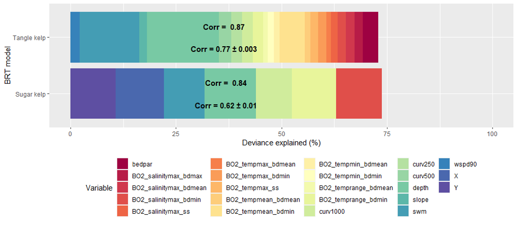
Figure 42. Evaluation statistics for the BRT models fitted for Norwegian data of sugar kelp (Saccharina) and tangle kelp (Laminaria). The models are evaluated by correlations (Corr) between model predictions and observations used for model building (training data) and from cross validation (for model testing with new data, CV). The color coding represents the fraction of total deviance explained by different explanatory variables. The deviance explained corresponds to the percentage of deviance for the null model (no pattern in the data) explained by the fitted model (100% for a perfect model).
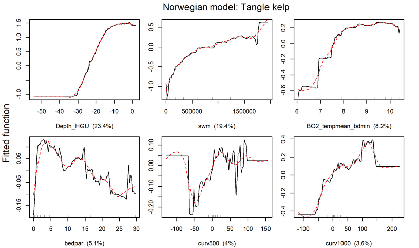
Figure 43. Partial dependence of tangle kelp density on predictor variables in the BRT model fitted for Norwegian data. The black lines show the marginal effect of the predictor variables on the response variable for the six most important variables (upper left to bottom right): bottom depth, wave exposure, mean temperature, PAR and bottom curvature with 500 m and 1 000 m spatial calculation window. The red lines give a smooth representation of the response, and the number in brackets indicates the contributions of the given variable.
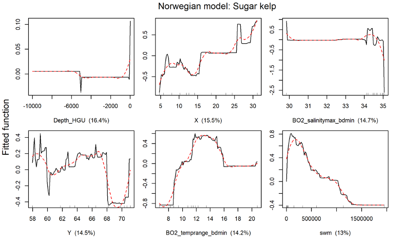
Figure 44. Partial dependence of sugar kelp density on predictor variables in the BRT model fitted for Norwegian data. The black lines show the marginal effect of the predictor variables on the response variable for the six most important variables (upper left to bottom right): bottom depth, longitude (X), maximum salinity, latitude (Y), temperature range, and wave exposure. The red lines give a smooth representation of the response, and the number in brackets indicates the contributions of the given variable. The importance of longitude and latitude reflects the fact that there is spatial variation that the given set of variables did not account for.
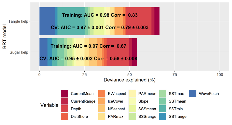
Figure 45. Evaluation statistics for the BRT models fitted for Nordic data of tangle kelp and sugar kelp. The models are evaluated by 1) the area under the curve (AUC) and 2) the correlation (Corr) between data and model predictions, where both metrics are calculated both from training data (data used for model building) and from cross validation (CV) (for model testing with new data, numbers given with standard error). The AUC ranges between 0 and 1, where a value of 0.5 indicates that the model predicts presence/absence no better than random, and a value of 1 indicates a perfect prediction. The color coding represents the fraction of total deviance explained by different explanatory variables. The deviance explained corresponds to the percentage of deviance for the null model (no pattern in the data) explained by the fitted model (100% for a perfect model).
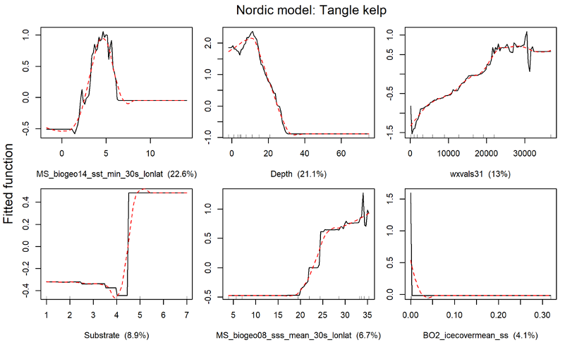
Figure 46. Partial dependence of presence of tangle kelp forest on predictor variables in the BRT model fitted for Nordic data. The black lines show the marginal effect of the predictor variables on the response variable for the six most important variables (upper left to bottom right): minimum sea surface temperature, bottom depth, wave fetch, substrate type, mean sea surface salinity and mean ice cover. The red lines give a smooth representation of the response, and the number in brackets indicates the contributions of the given variable.
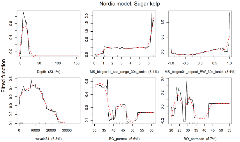
Figure 47. Partial dependence of presence of sugar kelp forest on predictor variables in the BRT model fitted for Nordic data. The black lines show the marginal effect of the predictor variables on the response variable for the six most important variables (upper left to bottom right): bottom depth, sea surface salinity range, east-west aspect, wave fetch, maximum and mean PAR. The red lines give a smooth representation of the response, and the number in brackets indicates the contributions of the given variable.
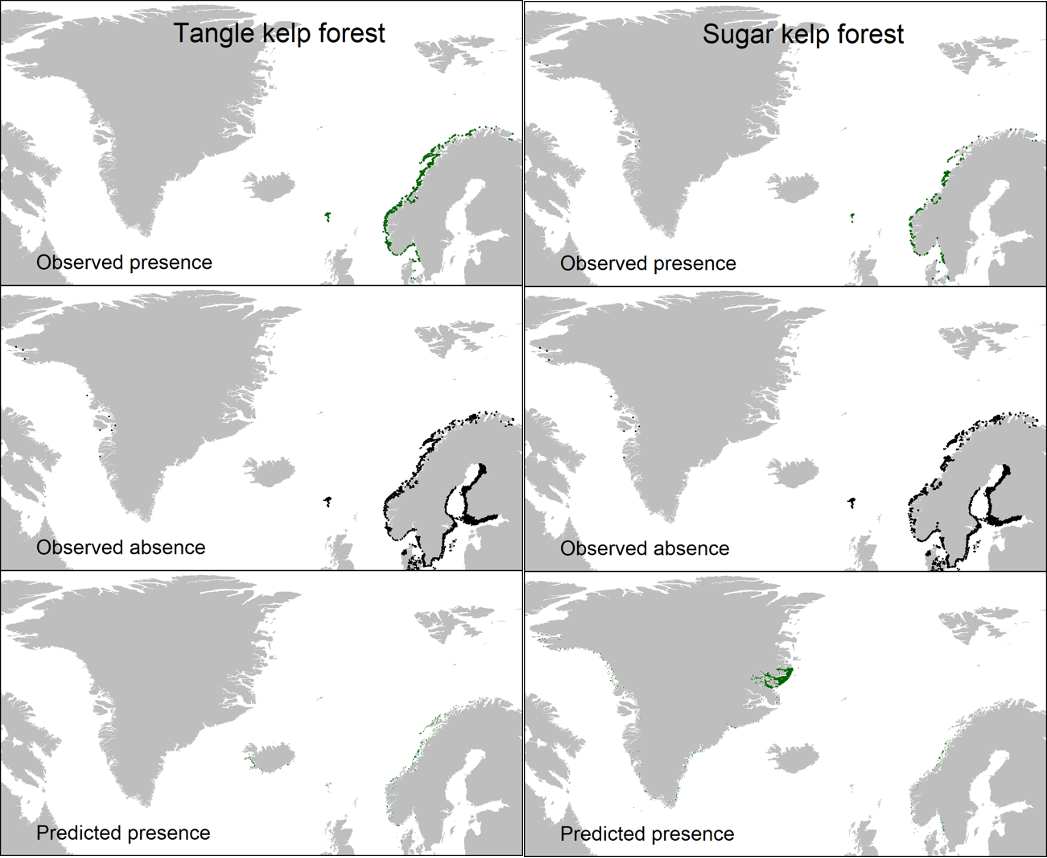
Figure 48. Distribution of compiled data for the Nordic countries on presence (upper) and absence (middle) of kelp forest, along with predicted presence (lower) of Laminaria spp. (left) and S. latissima (right) forests across the Nordic region. The green marking indicates predicted presence of forest within a grid cell (approximately 1 km resolution) and corresponds to Figure 7 in the main text.
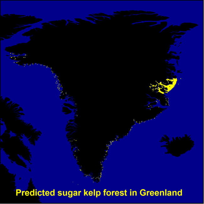
Figure 49. Predicted presence (yellow marking) of sugar kelp (Saccharina latissima or S. longicruris) forests in Greenland. The modelled presence is based on the probability models illustrated in Figure 5, and has a spatial resolution (grid cell size) of approximately 1 km. Predicted kelp forest areas north of 74°19 N on the east coast and north of 77°47 N on the west coast were removed because of lack of ground truth data for this region where extensive ice cover furthermore reduces the likelihood of abundant kelp forests (Dorte Krause-Jensen, personal observation).
Appendix B
Table 12. Compiled estimates entered in the carbon budget figures and Table 8 and Table 9, i.e. net primary production (NPP), exported and sequestered particulate organic carbon (POC) and dissolved organic carbon (DOC), and estimated carbon sequestration (POC+DOC) per unit habitat, and summarized for Norway, the Nordic region excluding Greenland, and Greenland. Carbon sequestration rates are also given in units of CO2 equivalents (million tonne CO2 equivalents year-1). Estimates are the predicted or weighted average of available data, see notes for details. The brackets indicate range (min-max) or standard deviation (SD).
| Habitat | Parameter | Unit | Kelp | SD | Min | Max | Rockweed | SD | Min | Max | Seagrass | SD |
| Per m2 habitat | NPP * | kg FW m-2 y-1 | 6.6 | 3.2 | 9.5 | 5.6 | 5.0 | |||||
| NPP, C units * | g C m-2 y-1 | 309 | 147 | 581 | 292 | 279 | 326 | 115 | ||||
| POC exported from beds/meadows ** | g C m-2 y-1 | 296 | 216 | 718 | 280 | 95 | 58 | 25 | ||||
| POC sequestered on the shelf *** | g C m-2 y-1 | 12.8 | 8 | 18 | 12.8 | - | ||||||
| POC sequestered in seagrass meadows **** | g C m-2 y-1 | - | - | 35 | 14 | |||||||
| POC exported to the deep sea ***** | g C m-2 y-1 | 7 | 0 | 15 | 7 | 0 | 15 | 9 | ||||
| DOC exported ¤ | g C m-2 y-1 | 155 | 62 | 371 | 58 | < 15 | 117 | 22 | ||||
| DOC exported below 1 000m ¤¤ | g C m-2 y-1 | 47 | 14 | 18 | 13 | 7 | ||||||
| Total sequestration ¤¤¤ | g C m-2 y-1 | 67.8 | 19 | 81 | 37.8 | 11 | 45 | 51 | 14 | |||
| Norway § | Area | km2 | 7 417 | 3 090 | 90 | |||||||
| NPP | million tonne FW y-1 | 49.3 | 24 | 70 | 17.2 | 0 | 0.5 | |||||
| NPP, C units | Gg C y-1 | 2 292 | 1 090 | 4 309 | 903 | 862 | 29 | 10 | ||||
| POC exported from beds/meadows | Gg C y-1 | 2 195 | 1 602 | 5 325 | 865 | 294 | 5 | 2.3 | ||||
| POC sequestered on the shelf | Gg C y-1 | 95 | 59 | 134 | 40 | - | ||||||
| POC sequestered in seagrass meadows | Gg C y-1 | 3.2 | 1.3 | |||||||||
| POC exported to the deep sea | Gg C y-1 | 53 | 0 | 115 | 21 | 0 | 45 | 0.8 | ||||
| DOC exported | Gg C y-1 | 1 146 | 458 | 2 750 | 181 | < 45 | 362 | 2.0 | ||||
| DOC exported below 1 000m | Gg C y-1 | 355 | 107 | 56 | 42 | 0.7 | ||||||
| Total sequestration | Gg C y-1 | 503 | 141 | 601 | 117 | 33 | 139 | 4.6 | 1.3 | |||
| Total sequestration | Mill tonne CO2 equiv. y-1 | 1.8 | 0.5 | 2.2 | 0.4 | 0.1 | 0.5 | 0.02 | 0.005 | |||
| Nordic § | Area | km2 | 10 990 | 5 556 | 2 611 | |||||||
| NPP | mill tonne FW y-1 | 73.0 | 35 | 104 | 30.9 | 13.2 | ||||||
| NPP, C units | Gg C y-1 | 3 396 | 1 616 | 6 385 | 1 624 | 1 552 | 850 | 300 | ||||
| POC exported from beds/meadows | Gg C y-1 | 3 253 | 2 374 | 7 891 | 1 556 | 528 | 151 | 65 | ||||
| POC sequestered on the shelf | Gg C y-1 | 141 | 88 | 198 | 71 | - | ||||||
| POC sequestered in seagrass meadows | Gg C y-1 | 92 | 37 | |||||||||
| POC exported to the deep sea | Gg C y-1 | 78 | 0 | 170 | 37 | 0 | 80 | 23 | ||||
| DOC exported | Gg C y-1 | 1 698 | 679 | 4 075 | 325 | < 81 | 650 | 57 | ||||
| DOC exported below 1000m | Gg C y-1 | 526 | 158 | 101 | 76 | 19 | ||||||
| Total sequestration | Gg C y-1 | 746 | 209 | 891 | 209 | 58 | 249 | 133 | 37 | |||
| Total sequestration | Million tonne CO2 equiv. y-1 | 2.7 | 0.8 | 3.2 | 0.8 | 0.2 | 0.9 | 0.48 | 0.13 | |||
| Greenland § | Area | km2 | 26 704 | |||||||||
| NPP | million tonne FW y-1 | 177.5 | 85 | 254 | ||||||||
| NPP, C units | Gg C y-1 | 8 252 | 3 925 | 15 515 | ||||||||
| POC exported from beds/meadows | Gg C y-1 | 7 904 | 5 768 | 19 173 | ||||||||
| POC sequestered on the shelf | Gg C y-1 | 342 | 214 | 481 | ||||||||
| POC sequestered in seagrass meadows | Gg C y-1 | |||||||||||
| POC exported to the deep sea | Gg C y-1 | 190 | 0 | 414 | ||||||||
| DOC exported | Gg C y-1 | 4 126 | 1 650 | 9 902 | ||||||||
| DOC exported below 1000m | Gg C y-1 | 1 279 | 384 | |||||||||
| Total sequestration | Gg C y-1 | 1 812 | 508 | 2 164 | ||||||||
| Total sequestration | Million tonne CO2 equiv. y-1 | 6.5 | 1.8 | 7.8 | ||||||||
| *) Norwegian kelp distribution/production model (this study) based on Abdullah & Fredriksen (2004), Pedersen et al. (2012, 2019), Sjøtun et al. (1995), rockweed from Pedersen et al. (2005), Krause-Jensen et al. (2012), Attard et al. (2018), Attard et al. (2019), seagrass from Krause-Jensen et al. (2012), Röhr et al. (2016), and refs herein. **) Kelp and rockweed POC export from algae beds to shelf and deep sea (Petersen et al., 2019; Pessarrodona et al., 2018), seagrass POC export from Duarte & Krause-Jensen (2017). ***) This study, Hardison et al. (2013), Krause-Jensen & Duarte (2016), and references herein for kelp and macroalgae. Assuming similar rates for rockweed. ****) Rohr et al. (2016) averaged for DK. *****) Kelp and macroalgae from Krause-Jensen & Duarte (2016), seagrass from Duarte and Krause-Jensen (2017). ¤) Kelp from this study (Ch. 2), Abdullah & Frederiksen (2004), Barrón et al. (2014), rockweed from Attard et al. (2018), Sieburth (1969), Carlson and Carlson (1984), Maher and Eyre (2010), Krause-Jensen & Duarte (2016), seagrass from Duarte and Krause-Jensen (2017). ¤¤) Kelp and rockweed from Krause-Jensen (2016) and references herein, seagrass from Duarte and Krause-Jensen (2017) and references herein. ¤¤¤) Total carbon sequestration is the sum of POC sequestered on the shelf and in meadows, POC exported to the deep sea (below 1 000 m), and DOC exported below 1 000 m (below the mixed ocean layer). § See Chapter 1 for uncertainty estimates on the areal coverage data. | ||||||||||||
Appendix C
Table 13. Overview of literature that was used as the basis for discussions with the work group to draw up the schematic presentations of the ecological networks. These served as input to the analyses of ecosystem stability and pressure responses (impacts of climate change, eutrophication, overfishing and management measures).
| Title | Year | System(s) | Interactions described ± and comments | Full reference |
| A cross-scale trophic cascade from large predatory fish to algae in coastal ecosystems | 2017 | Rockweed communities | Piscivores (perch and pike) --* mesopredators (three-spined sticklebacks) Three-spined sticklebacks --* epifaunal grazers Grazers --* epiphytes Habitat-forming veg. --> grazers | Donadi, S., Austin, Å.N., Bergström, U., Eriksson, B.K., Hansen, J.P., Jacobson, P., Sundblad, G., Van Regteren, M. and Eklöf, J.S., 2017. A cross-scale trophic cascade from large predatory fish to algae in coastal ecosystems. Proceedings of the Royal Society B: Biological Sciences, 284(1859), p.20170045. |
| A three-stage symbiosis forms the foundation of seagrass ecosystems | 2012 | Seagrass meadows | Gill bacteria (sulfide oxidizing) <---> Seagrass | van der Heide, T., Govers, L.L., de Fouw, J., Olff, H., van der Geest, M., van Katwijk, M.M., Piersma, T., van de Koppel, J., Silliman, B.R., Smolders, A.J. and van Gils, J.A., 2012. A three-stage symbiosis forms the foundation of seagrass ecosystems. Science, 336(6087), pp.1432-1434. |
| Confronting feedbacks of degraded marine ecosystems | 2012 | Kelp forest, Seagrass meadows, Rockweed communities | A general picture of feedback mechanisms in different marine systems, very general but useful | Nyström, M., Norström, A.V., Blenckner, T., de la Torre-Castro, M., Eklöf, J.S., Folke, C., Österblom, H., Steneck, R.S., Thyresson, M. and Troell, M., 2012. Confronting feedbacks of degraded marine ecosystems. Ecosystems, 15(5), pp. 695-710. |
| Cover of coastal vegetation as an indicator of eutrophication along environmental gradients | 2016 | Kelp forest, Seagrass meadows, Rockweed communities | Eutrophication ---* macrophyte cover Water clarity ---> macrophyte cover | Wikström, S.A., Carstensen, J., Blomqvist, M. and Krause-Jensen, D., 2016. Cover of coastal vegetation as an indicator of eutrophication along environmental gradients. Marine biology, 163(12), p. 257. |
| Declines in predatory fish promote bloom‐forming macroalgae | 2009 | Rockweed communities | Large predatory fish ---* smaller predatory fish Juvenile large pred. fish *---* smaller pred. fish (suggested competitive) Smaller predatory fish ---* herbivores Herbivores ---* ephemeral algae Nutrients ---> ephemeral algae (additive) Ephemeral algae ---> herbivores (when large predators excluded) Herbivores ---> smaller predatory fish (when large predators excluded) Canopy ---> herbivores (suggested) Canopy ---* ephemeral algae (shading, whiplash?) | Eriksson, B.K., Ljunggren, L., Sandström, A., Johansson, G., Mattila, J., Rubach, A., Råberg, S. and Snickars, M., 2009. Declines in predatory fish promote bloom‐forming macroalgae. Ecological Applications, 19(8), pp. 1975-1988. |
| Distribution of mesopredatory fish determined by habitat variables in a predator-depleted coastal system | 2016 | Seagrass meadows, Rockweed communities | Habitat quality (structure, high cover of large habitat-forming vegetation) ---> mesopredatory fish | Bergström, L., Karlsson, M., Bergström, U., Pihl, L. and Kraufvelin, P., 2016. Distribution of mesopredatory fish determined by habitat variables in a predator-depleted coastal system. Marine biology, 163(10), p. 201. |
| Distribution, structure and function of Nordic eelgrass (Zostera marina) ecosystems: implications for coastal management and conservation | 2014 | Seagrass meadows | Trophic cascades and bottom-up (species on all levels are mentioned) | Boström, C., Baden, S., Bockelmann, A.C., Dromph, K., Fredriksen, S., Gustafsson, C., Krause‐Jensen, D., Möller, T., Nielsen, S.L., Olesen, B. and Olsen, J., 2014. Distribution, structure and function of Nordic eelgrass (Zostera marina) ecosystems: implications for coastal management and conservation. Aquatic conservation: marine and freshwater ecosystems, 24(3), pp. 410-434. |
| Eelgrass (Zostera marina) food web structure in different environmental settings | 2016 | Seagrass meadows | Describing differences in food web structures. As expected. Could be used to validate models? | Thormar, J., Hasler-Sheetal, H., Baden, S., Boström, C., Clausen, K.K., Krause-Jensen, D., Olesen, B., Rasmussen, J.R., Svensson, C.J. and Holmer, M., 2016. Eelgrass (Zostera marina) food web structure in different environmental settings. PLoS One, 11(1), p.e0146479. |
| Eelgrass Zostera marina in subarctic Greenland: dense meadows with slow biomass turnover in cold waters | 2015 | Seagrass meadows | Temperature (when cold) --> eelgrass growth and reproduction (distribution and production in cold areas predicted to increase in a warmer future) | Olesen, B., Krause-Jensen, D., Marbà, N. and Christensen, P.B., 2015. Eelgrass Zostera marina in subarctic Greenland: dense meadows with slow biomass turnover in cold waters. Marine Ecology Progress Series, 518, pp. 107-121. |
| Future warming and acidification effects on anti‐fouling and anti‐herbivory traits of the brown alga Fucus vesiculosus (Phaeophyceae) | 2016 | Rockweed communities | Warming ---> grazing (on both fucoid host and epiphytes) | Raddatz, S., Guy‐Haim, T., Rilov, G. and Wahl, M., 2017. Future warming and acidification effects on anti‐fouling and anti‐herbivory traits of the brown alga Fucus vesiculosus (Phaeophyceae). Journal of Phycology, 53(1), pp. 44-58. |
| Global patterns of kelp forest change over the past half-century | 2016 | Kelp forest | Globally comprehensive analysis of kelp forest change over the past 50 y, identifying a high degree of variation in the magnitude and direction of change across the geographic range of kelps. These results suggest region-specific responses to global change, with local drivers playing an important role in driving patterns of kelp abundance. | Krumhansl, K.A., Okamoto, D.K., Rassweiler, A., Novak, M., Bolton, J.J., Cavanaugh, K.C., Connell, S.D., Johnson, C.R., Konar, B., Ling, S.D. and Micheli, F., 2016. Global patterns of kelp forest change over the past half-century. Proceedings of the National Academy of Sciences, 113(48), pp. 13785-13790. |
| Importance of genetic diversity in eelgrass Zostera marina for its resilience to global warming | 2008 | Seagrass meadows | Genotypic diversity important for resilience | Ehlers, A., Worm, B. and Reusch, T.B., 2008. Importance of genetic diversity in eelgrass Zostera marina for its resilience to global warming. Marine Ecology Progress Series, 355, pp. 1-7. |
| In situ warming strengthens trophic cascades in a coastal food web | 2017 | Rockweed communities | High temperature --* small mesopredatory fish Predatory fish <--* small mesopredatory fish Predatory fish <--* mesograzers (when high temperature) (feeding on lower trophic levels compressing chain) NB! mesograzers <--* filamentous algae Could be used to validate models? Increased temperature benefited filamentous algae by releasing the pressure from mesograzers (due to increased predation from larger predators even though the abundance of smaller predatory fish declined in heated areas) | Svensson, F., Karlsson, E., Gårdmark, A., Olsson, J., Adill, A., Zie, J., Snoeijs, P. and Eklöf, J.S., 2017. In situ warming strengthens trophic cascades in a coastal food web. Oikos, 126(8), pp. 1150-1161. |
| Intra-and interspecific differences in palatability of Arctic macroalgae from Kongsfjorden (Spitsbergen) for two benthic sympatric invertebrates | 2006 | Rockweed communities | Green sea urchin Strongylocentrotus droebachiensis (OF Müller) and the amphipod Gammarellus homari (JC Fabricius) ---* perennial "leathery" and foliose macroalgae (e.g. Palmaria, Laminaria, Alaria) as opposed to e.g. Desmarestia and Ptilota (strong - esp. urchin grazing) D. ramentacea ---> G. homari (food and shelter) (suggested) | Wessels, H., Hagen, W., Molis, M., Wiencke, C. and Karsten, U., 2006. Intra-and interspecific differences in palatability of Arctic macroalgae from Kongsfjorden (Spitsbergen) for two benthic sympatric invertebrates. Journal of experimental marine biology and ecology, 329(1), pp. 20-33. |
| Long-term decline and recent recovery of Fucus populations along the rocky shores of southeast Sweden, Baltic Sea | 2004 | Rockweed communities | Idotea baltica (isopod) ---* Fucus spp. (strong) (grazing) Positive effects of temperature (mild) and eutrophication on I. baltica discussed, but not really investigated. Likewise; Fish predation (e.g. cod and herring) ---* I. baltica (suggested) | Nilsson, J., Engkvist, R. and Persson, L.E., 2004. Long-term decline and recent recovery of Fucus populations along the rocky shores of southeast Sweden, Baltic Sea. Aquatic Ecology, 38(4), pp. 587-598. |
| Metabolomics reveals cryptic interactive effects of species interactions and environmental stress on nitrogen and sulfur metabolism in seagrass | 2016 | Seagrass meadows | Blue mussels (high light) ---> seagrass (stimulate nitrogen metabolism) Blue mussels (low light) ---* seagrass (drained oxygen levels close to the sediment surface, enhancing the potential for sulfide intrusion leading to sulfide toxicity. | Hasler-Sheetal, H., Castorani, M.C., Glud, R.N., Canfield, D.E. and Holmer, M., 2016. Metabolomics reveals cryptic interactive effects of species interactions and environmental stress on nitrogen and sulfur metabolism in seagrass. Environmental science & technology, 50(21), pp. 11602-11609. |
| Predators of the destructive sea urchin grazer Strongylocentrotus droebachiensis on the Norwegian coast | 2014 | Kelp forest | Crab (Cancer pagurus and Carcinus maenas) ---* sea urchin (Strongylocentrotus droebachiensis) (strong) Other decapod crustaceans ---* sea urchin (intermediate) Sea urchin ---* kelp (Laminaria hyperborea) (Norderhaug & Christie 2009) (very strong) Increased ocean temperature ---* recruitment of sea urchin (Fagerli et al., 2013) (?) Increased ocean temperature ---> Cancer pagurus (?) | Norderhaug, K.M., Christie, H.C., Pedersen, M.F. and Fredriksen, S., 2014. Predators of the destructive sea urchin grazer Strongylocentrotus droebachiensis on the Norwegian coast. |
| Recovery of Danish coastal ecosystems after reductions in nutrient loading: a holistic ecosystem approach | 2016 | Seagrass meadows, Rockweed communities | Expected links, also discuss management framework NB!! Could be used to validate models? | Riemann, B., Carstensen, J., Dahl, K., Fossing, H., Hansen, J.W., Jakobsen, H.H., Josefson, A.B., Krause-Jensen, D., Markager, S., Stæhr, P.A. and Timmermann, K., 2016. Recovery of Danish coastal ecosystems after reductions in nutrient loading: a holistic ecosystem approach. Estuaries and Coasts, 39(1), pp. 82-97. |
| Responses of marine organisms to climate change across oceans | 2016 | Lots, but few details | Poloczanska, E.S., Burrows, M.T., Brown, C.J., García Molinos, J., Halpern, B.S., Hoegh-Guldberg, O., Kappel, C.V., Moore, P.J., Richardson, A.J., Schoeman, D.S. and Sydeman, W.J., 2016. Responses of marine organisms to climate change across oceans. Frontiers in Marine Science, 3, p. 62. | |
| Responses to nutrient enrichment, wave action and disturbance in rocky shore communities | 2007 | Rockweed communities | Disturbance of seaweed (scraping) ---> Filamentous red and brown algae +++Nutrients ---> green foliose algae Green foliose algae *---* Filamentous red and brown algae (competitive) +++Nutrients --->grazers (esp. Gammarus (amphipod) and Jaera (isopod)) (increased food availability?) | Kraufvelin, P., 2007. Responses to nutrient enrichment, wave action and disturbance in rocky shore communities. Aquatic Botany, 87(4), pp. 262-274. |
| Role of biological habitat amelioration in altering the relative responses of congeneric species to climate change | 2007 | Rockweed communities | Fucus spp ---> Patella vulgata (shelter and food) Patella vulgata ---* macroalgae (grazing) (mentioned, should be able to get a reference) Temperature ---* Fucus spp ---* P. vulgata (predicted) | Moore, P., Hawkins, S.J. and Thompson, R.C., 2007. Role of biological habitat amelioration in altering the relative responses of congeneric species to climate change. Marine Ecology Progress Series, 334, pp. 11-19. |
| Season exerts differential effects of ocean acidification and warming on growth and carbon metabolism of the seaweed Fucus vesiculosus in the western Baltic Sea | 2015 | Rockweed communities | Heat wave --* Fucus --> Filamentous algae | Graiff, A., Bartsch, I., Ruth, W., Wahl, M. and Karsten, U., 2015. Season exerts differential effects of ocean acidification and warming on growth and carbon metabolism of the seaweed Fucus vesiculosus in the western Baltic Sea. frontiers in Marine Science, 2, p. 112. |
| Shifts in coastal fish communities: Is eutrophication always beneficial for sticklebacks? | 2017 | Rockweed communities | Predatory fish ---* mesopredators | Gagnon, K., Gräfnings, M. and Boström, C., 2017. Shifts in coastal fish communities: Is eutrophication always beneficial for sticklebacks? Estuarine, Coastal and Shelf Science, 198, pp. 193-203. |
| Synergistic effects of climate change and local stressors: CO2 and nutrient‐driven change in subtidal rocky habitats | 2009 | Kelp forest | (Australia) Nutrients ---> Turfs CO2/acidification ---> Turfs Temperature ---> Turfs Turf *---* Kelp/understory veg. (shown elsewhere) | Russell, B.D., Thompson, J.A.I., Falkenberg, L.J. and Connell, S.D., 2009. Synergistic effects of climate change and local stressors: CO2 and nutrient‐driven change in subtidal rocky habitats. Global Change Biology, 15(9), pp. 2153-2162. |
| The funda|mental role of eco|logi|cal feed|back mecha|nisms for the adap|tive manage|ment of sea|grass eco|systems - a review | 2016 | Seagrass meadows | Seagrass ---> seagrass (slows water flow - protects against physical stress from water drag, retains particles - improving light cond. and growth, stabilizing the sea floor, oxygenating sediments alleviating the toxic effect of e.g. sulfide build-up) Reduced water flow ---* deposit of organic matter may improve growth when low (in oligotrophic systems). When high, can lead to sulphide toxicity, which impairs shoot density and growth. Lucinid bivalves (and their gill bacteria) <---> seagrass (lucinid bivalves benefit from organic buildup and oxygenated sediments near the rhizomes. These in turn reduce the sulfide levels, improving the conditions for the seagrass) Algae (epi, turfs, mats, planktonic) ---* Seagrass (compete for light and space) Seagrass ---> mezograzers Mezograzers ---* epiphytes/turfs Multiple trophic cascades... Eutrophication (hypoxia or anoxia) ---* Grazers | Maxwell, P.S., Eklöf, J.S., van Katwijk, M.M., O'Brien, K.R., de la Torre‐Castro, M., Boström, C., Bouma, T.J., Krause‐Jensen, D., Unsworth, R.K., van Tussenbroek, B.I. and van der Heide, T., 2017. The fundamental role of ecological feedback mechanisms for the adaptive management of seagrass ecosystems–a review. Biological Reviews, 92(3), pp. 1521-1538. |
| The influence of physical factors on kelp and sea urchin distribution in previously and still grazed areas in the NE Atlantic | 2014 | Kelp forest | Wave exposure (< a certain point) and salinity ---> kelp recovery (strong) Wave exposure ---* urchin persistence (strong) Mean August temperature (< 12 C) ---> Kelp recovery (strong) Mean August temperature ---* urchin persistence (strong) (Fresher water ---* urchin persistence ?) Depth ---* kelp recovery (related to light) Depth ---* sea urchin persistence Currents (< a certain point) ---> kelp recovery Currents ---> urchin persistence (strong) Slope (< 10-15 deg) ---> kelp recovery (related to light, sedimentation and substrate as well...) | Rinde, E., Christie, H., Fagerli, C.W., Bekkby, T., Gundersen, H., Norderhaug, K.M. and Hjermann, D.Ø., 2014. The influence of physical factors on kelp and sea urchin distribution in previously and still grazed areas in the NE Atlantic. PLoS One, 9(6), p.e100222. |
| Top-down control as important as nutrient enrichment for eutrophication effects in North Atlantic coastal ecosystems | 2016 | Seagrass meadows, Rockweed communities | Conceptual web described | Östman, Ö., Eklöf, J., Eriksson, B.K., Olsson, J., Moksnes, P.O. and Bergström, U., 2016. Top‐down control as important as nutrient enrichment for eutrophication effects in North Atlantic coastal ecosystems. Journal of Applied Ecology, 53(4), pp. 1138-1147. |
SEAGRASS SYSTEMS – PRESSURE RESPONSE FIGURES
Figure 50. Pressure responses in the seagrass systems when exposed to climate change (increases in temperature and sedimentation and reductions in light).
Figure 51. Pressure responses in the seagrass systems when exposed to climate change, overfishing and eutrophication.
Figure 52. Pressure responses in the seagrass systems when exposed to climate change and management efforts to reduce nutrients.
Figure 53. Pressure responses in the seagrass systems when exposed to climate change and management efforts to improve light conditions.
Figure 54. Pressure responses in the seagrass systems when exposed to climate change and management efforts to reduce sedimentation.
Figure 55. Pressure responses in the seagrass systems when exposed to climate change and management efforts to reduce fishing pressure.
Figure 56. Pressure responses in seagrass systems when exposed to climate change and a full range of management measures (aimed at reducing sedimentation, nutrient loadings and fishing pressure, and improving light conditions).
ROCKWEED (WRACK) SYSTEMS – PRESSURE RESPONSE FIGURES
Figure 57. Pressure responses in the rockweed (wrack) systems when exposed to climate change (increases in temperature and sedimentation and reductions in light).
Figure 58. Pressure responses in the rockweed (wrack) systems when exposed to climate change, including increased scouring.
Figure 59. Pressure responses in the rockweed (wrack) systems when exposed to climate change, including decreased scouring.
Figure 60. Pressure responses in the rockweed (wrack) systems when exposed to climate change, overfishing and eutrophication.
Figure 61. Pressure responses in the rockweed (wrack) systems when exposed to climate change and management efforts to improve light conditions.
Figure 62. Pressure responses in the rockweed (wrack) systems when exposed to climate change and management efforts to reduce nutrients.
Figure 63. Pressure responses in the rockweed (wrack) systems when exposed to climate change and management efforts to reduce sedimentation.
Figure 64. Pressure responses in the rockweed (wrack) systems when exposed to climate change and management efforts to reduce fishing pressure.
Figure 65. Pressure responses in the rockweed (wrack) systems when exposed to climate change and a full range of management measures (aimed at reducing sedimentation, nutrient loadings and fishing pressure, and improving light conditions).
L. HYPERBOREA SYSTEMS – PRESSURE RESPONSE FIGURES
Figure 66. Pressure responses in the tangle kelp (Laminaria hyperborea) systems when exposed to climate change (increases in temperature and sedimentation and reductions in light).
Figure 67. Pressure responses in the tangle kelp (Laminaria hyperborea) systems when exposed to climate change, overfishing and eutrophication.
Figure 68. Pressure responses in the tangle kelp (Laminaria hyperborea) systems when exposed to climate change and management efforts to reduce nutrients.
Figure 69. Pressure responses in the tangle kelp (Laminaria hyperborea) systems when exposed to climate change and management efforts to improve light conditions.
Figure 70. Pressure responses in the tangle kelp (Laminaria hyperborea) systems when exposed to climate change and management efforts to reduce fishing pressure.
Figure 71. Pressure responses in the tangle kelp (Laminaria hyperborea) systems when exposed to climate change and management efforts to reduce the pressure from urchins.
Figure 72. Pressure responses in the tangle kelp (Laminaria hyperborea) systems when exposed to climate change and a full range of management measures (aimed at reducing sedimentation, nutrient loadings, fishing pressure and pressure from urchins, and improving light conditions).
About this publication
Blue Carbon – climate adaptation, CO2 uptake and sequestration of carbon in Nordic blue forests
Results from the Nordic Blue Carbon Project
Helene Frigstad, Hege Gundersen, Guri S. Andersen, Gunhild Borgersen, Kristina Ø. Kvile, Dorte Krause-Jensen, Christoffer Boström, Trine Bekkby, Marc Anglès d'Auriac, Anders Ruus, Jonas Thormar, Kaya Asdal and Kasper Hancke
ISBN 978-92-893-6860-5 (PDF)
ISBN 978-92-893-6861-2 (ONLINE)
http://dx.doi.org/10.6027/temanord2020-541
TemaNord 2020:541
ISSN 0908-6692
Cover photo: Rune E. Haldorsen
© Nordic Council of Ministers 2020
Disclaimer
This publication was funded by the Nordic Council of Ministers. However, the content does not necessarily reflect the Nordic Council of Ministers’ views, opinions, attitudes or recommendations.
Rights and permissions
This work is made available under the Creative Commons Attribution 4.0 International license (CC BY 4.0) https://creativecommons.org/licenses/by/4.0.
Translations: If you translate this work, please include the following disclaimer: This translation was not produced by the Nordic Council of Ministers and should not be construed as official. The Nordic Council of Ministers cannot be held responsible for the translation or any errors in it.
Adaptations: If you adapt this work, please include the following disclaimer along with the attribution: This is an adaptation of an original work by the Nordic Council of Ministers. Responsibility for the views and opinions expressed in the adaptation rests solely with its author(s). The views and opinions in this adaptation have not been approved by the Nordic Council of Ministers.
Third-party content: The Nordic Council of Ministers does not necessarily own every single part of this work. The Nordic Council of Ministers cannot, therefore, guarantee that the reuse of third-party content does not infringe the copyright of the third party. If you wish to reuse any third-party content, you bear the risks associated with any such rights violations. You are responsible for determining whether there is a need to obtain permission for the use of third-party content, and if so, for obtaining the relevant permission from the copyright holder. Examples of third-party content may include, but are not limited to, tables, figures or images.
Photo rights (further permission required for reuse):
Any queries regarding rights and licences should be addressed to:
Nordic Council of Ministers/Publication Unit
Ved Stranden 18
DK-1061 Copenhagen
Denmark
pub@norden.org
Nordic co-operation
Nordic co-operation is one of the world’s most extensive forms of regional collaboration, involving Denmark, Finland, Iceland, Norway, Sweden, and the Faroe Islands, Greenland and Åland.
Nordic co-operation has firm traditions in politics, economics and culture and plays an important role in European and international forums. The Nordic community strives for a strong Nordic Region in a strong Europe.
Nordic co-operation promotes regional interests and values in a global world. The values shared by the Nordic countries help make the region one of the most innovative and competitive in the world.
The Nordic Council of Ministers
Nordens Hus
Ved Stranden 18
DK-1061 Copenhagen
pub@norden.org
Read more Nordic publications on www.norden.org/publications